First simulation¶

This page builds and runs exec/_Tests/Advection, looks at the output, and runs the same problem with THINC and with Phase-Field regularization. It assumes COMPAS and AMReX are cloned side by side as in Installation.

The case uses the two-phase five-equation model (FIVEEQS) in 2D. A slotted disk, a square, a circle and a triangle of material 2, each with its own density, are carried through material 1 at the uniform velocity \((1,1)\) across the periodic box \([-1,1]^2\). The run stops after one period, at stop_time = 2.0, when the exact solution is the initial condition again. The base grid has 64 by 64 cells, with two levels of refinement that follow the interfaces.

Build¶

cd COMPAS/exec/_Tests/Advection
make -j4

The last lines of the build show the model options and the executable:

mpicxx ... -DPHYSICS=FIVEEQS -DADVECTION=true -DDIFFUSION=false -DNONCONSERVATIVE=true ...
       ... -o main2d.gnu.MPI.ex ...
SUCCESS

How the name main2d.gnu.MPI.ex encodes the build is explained in Installation.

Run¶

mpirun -n 4 ./main2d.gnu.MPI.ex prob/inputs amr.plot_int=50

The first argument is the inputs file, and anything after it overrides a parameter of that file: here amr.plot_int adds a plotfile every 50 coarse steps to the ones written every 0.1 time units (amr.t_write_interval). The run takes about 15 seconds on four cores.

Each coarse step prints the steps taken on every level and a short summary:

==== Coarse step 440 ====
[Level 0 step 440]           Advance with time = 1.997979765 dt = 0.002020235487 ==> Advanced 4096 cells
    [Level 1 step 879]       Advance with time = 1.997979765 dt = 0.001010117743 ==> Advanced 16384 cells
        [Level 2 step 1757]   Advance with time = 1.997979765 dt = 0.0005050588717 ==> Advanced 44032 cells
        [Level 2 step 1758]   Advance with time = 1.998484823 dt = 0.0005050588717 ==> Advanced 44032 cells
    ...
[COMPAS] Coarse step:     440
           SimulationTime:  2
           Timestep:        0.002020235487
           SumVar:          a1rho1
           Sum:             3260.499661
           ...

With run.do_subcycle = 1, each finer level takes two steps of half the size for every step of the level below. Sum, turned on or off with run.timestep_sum, is the sum over the domain of the variable chosen by run.sum_var, here the partial density \(\alpha_1\rho_1\), a quick conservation check (Output).

A serial build (make USE_MPI=FALSE) produces main2d.gnu.ex, which runs without mpirun.

What a run writes¶

The output goes where amr.case_name = ./plot/Advection5Eq says:

plot/Advection5Eq/
├── config_log_Advection5Eq.txt   everything needed to reproduce the run
├── Advection5Eq.visit            the plotfiles as a time series, for VisIt
├── advection.csv                 diagnostics written by this case every coarse step
├── plt_Advection5Eq00000/        one plotfile, named by the coarse step
│   ├── Header                    variables, time and grids
│   ├── Level_0/                  data on each AMR level
│   ├── Level_1/
│   └── Level_2/
├── plt_Advection5Eq00022/
└── ...
checkpoints/
├── chk00000/                     for restarts, set by amr.chk_file and amr.chk_int
└── chk00440/

The configuration log records the AMReX version, the number of MPI ranks, every run-time parameter, from the inputs file, the command line or the AMReX defaults, and copies of prob/ProblemICBC.H, prob/inputs, prob/Parm.H and GNUmakefile:

=====================================================================
 COMPAS CONFIGURATION LOG
 Created: ...
 Output Directory: ./plot/Advection5Eq
---------------------------------------------------------------------
 MPI Ranks: 4
=====================================================================

================ AMReX Build Information ================
AMReX Version: 26.01
...
================ Runtime Parameters ================
...
FiniteVolume.Scheme(nvals = 1)  :: [MUSCL-MC]
...

advection.csv comes from the UserOutputFunction of this case, called every coarse step because run.user_output_int = 1. It holds the area of material 2, the extrema of \(\alpha_1\), the largest departures of pressure and velocity from their uniform initial values, and N_I, the thickness of the interfaces in finest cells (prob.interface_thickness = 1). Writing such a function is described in Setting up a case.

bash ../../clean.sh removes the plotfiles and checkpoints of previous runs.

Look at the results¶

ParaView and VisIt open a plt* directory as an AMReX plotfile. In VisIt, the .visit file loads the whole run as a time series.

yt reads plotfiles directly from Python. With the environment from Installation active, from the case directory:

import yt
ds = yt.load("plot/Advection5Eq/plt_Advection5Eq00440")
print(ds.field_list)   # [('boxlib', 'P'), ('boxlib', 'a1'), ('boxlib', 'a1rho1'), ('boxlib', 'rho'), ...]
yt.SlicePlot(ds, "z", ("boxlib", "rho")).save()

The fields are the variables listed in run.output_vars. plt_Advection5Eq00440 is the last plotfile of the run, at \(t = 2\).

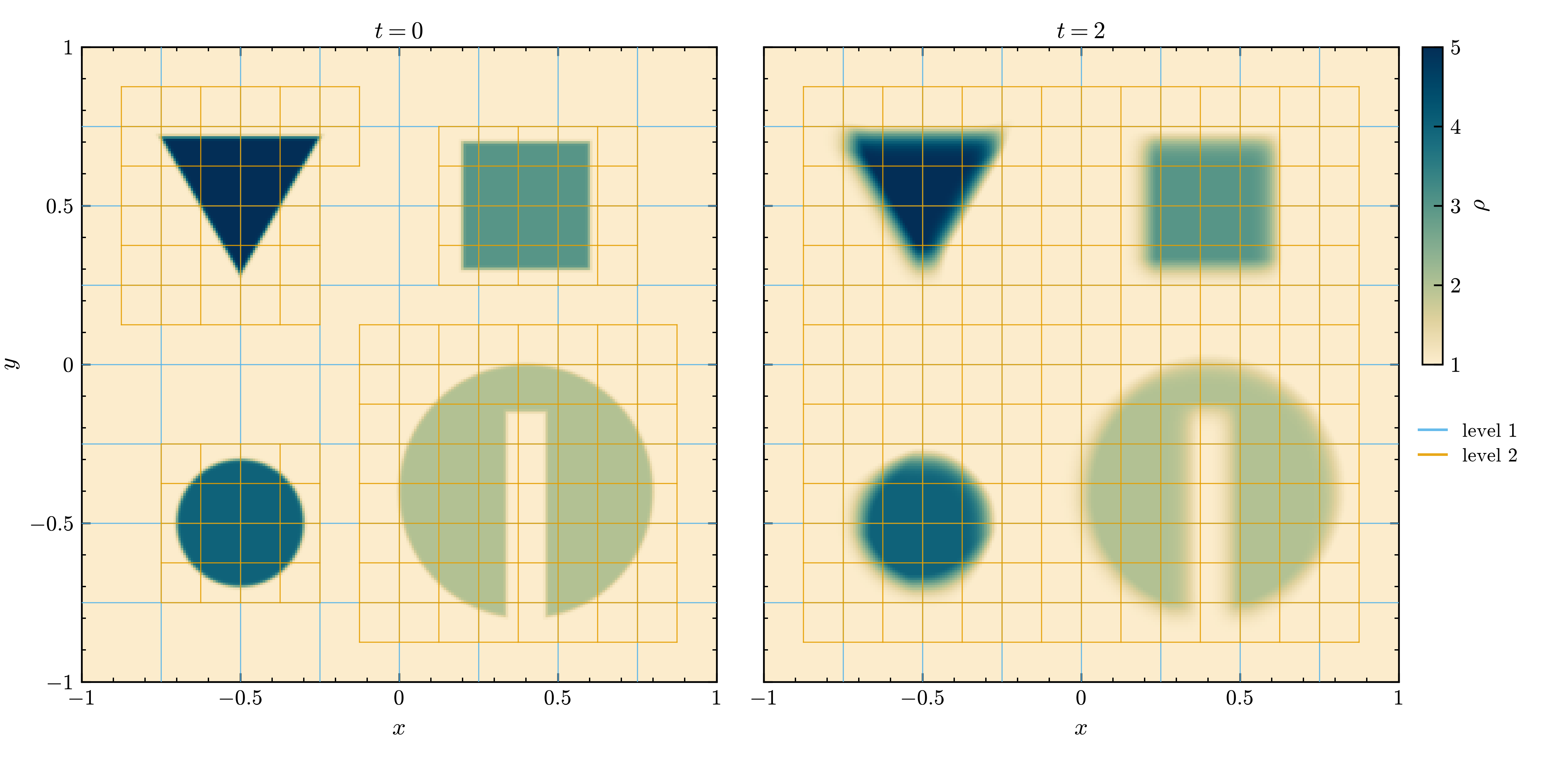
Density of Advection-5Eq at t = 0 and t = 2

Density \(\rho\) of Advection-5Eq at \(t = 0\) and after one period, \(t = 2\), with the patches of AMR levels 1 (blue) and 2 (orange), which follow the interfaces.

The columns of advection.csv can be plotted with scripts/plot.py, which sets up the Python environment by itself on first use:

python3 ../../../scripts/plot.py --csv plot/Advection5Eq/advection.csv --x t --y V_2

scripts/postprocess.py draws the plotfiles as snapshot figures and movies (Post-processing script), for example the volume fraction at the start and after one period, with the AMR levels outlined:

python3 ../../../scripts/postprocess.py snapshots plot/Advection5Eq --times 0 2 --amr

Try THINC and Phase-Field¶

The same problem is provided with the two interface treatments, as two more inputs files for the same executable:

mpirun -n 4 ./main2d.gnu.MPI.ex prob/inputs.Advection-THINC-5Eq     # THINC reconstruction
mpirun -n 4 ./main2d.gnu.MPI.ex prob/inputs.Advection-PF-5Eq        # Phase-Field regularization

They write to plot/Advection5Eq-THINC/ and plot/Advection5Eq-PF/, with the same columns in advection.csv, so N_I compares the interface thickness of the three methods. The methods are switched on in the inputs files:

FiniteVolume.THINC       = 1           # Advection-THINC-5Eq

PhaseField.phase_field   = 1           # Advection-PF-5Eq
PhaseField.Mechanism     = "CAC-Adv"
PhaseField.ID_ExplicitRC = 0           # implicit

The THINC run takes about as long as the first one. The Phase-Field run solves an implicit system every step and takes about a minute on four cores.

The three results are compared under Interface advection.

Change methods on the command line¶

Any parameter of the inputs file can be overridden at launch, so comparing methods needs no rebuild and no edit of prob/inputs. From exec/_Tests/Advection:

./main2d.gnu.MPI.ex prob/inputs FiniteVolume.Scheme=WENO5 Physics.RiemannSolver=HLL
./main2d.gnu.MPI.ex prob/inputs PhaseField.phase_field=1 PhaseField.Mechanism=ACDI PhaseField.ID_ExplicitRC=1
./main2d.gnu.MPI.ex prob/inputs amr.max_level=0 stop_time=0.5

Prefix them with mpirun -n 4 to run in parallel. Add amr.case_name=./plot/MyRun to keep the output of a variant apart from the base run.

A value COMPAS does not recognize stops the run at startup and lists the valid values:

$ ./main2d.gnu.MPI.ex prob/inputs run.TimeIntegrator=SSPRK3
amrex::Abort::0::run.TimeIntegrator = 'SSPRK3' is not recognized. Valid values are ForwardEuler, TVD-RK2, TVD-RK3, RK4. !!!

At the end of a run, AMReX lists the parameters that were set but never read, so a misspelled name shows up there. Every entry of this case’s inputs file is read, so the list appears only after a mistake, such as FiniteVolume.Schem=WENO5 on the command line:

Unused ParmParse Variables:
  [TOP]::FiniteVolume.Schem(nvals = 1)  :: [WENO5]

All the run-time parameters and their values are listed in Run-time options.