Verification and validation

This page compares COMPAS with exact solutions, theory and experiments. Each section names the case that produces it. The methods of a case are set in its prob/inputs, and the commands below show only what a run changes. The test suite described in Testing is a separate build-and-stability check.

Shock tubes

Sod shock tube

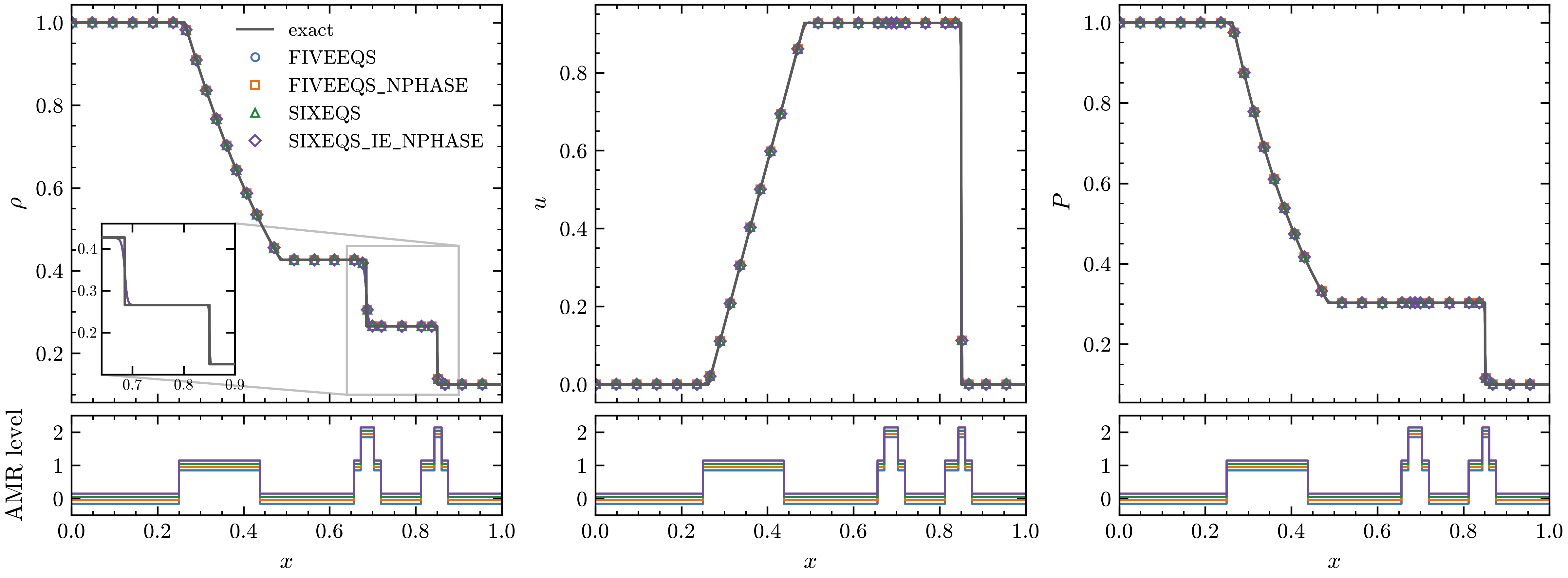
Sod shock tube at \(t = 0.2\) with the four models and the exact solution (gray line): density \(\rho\), velocity \(u\) and pressure \(P\). The inset enlarges the contact and the shock. The strip under each panel gives the finest AMR level along \(x\) for each model, offset slightly so the four can be told apart.

The shock tube of Sod (J. Comput. Phys. 27, 1978) starts from gas at rest with \(\rho = 1\), \(P = 1\) for \(x < 0.5\) and \(\rho = 0.125\), \(P = 0.1\) beyond, with \(\gamma = 1.4\). exec/_Tests/Sod runs it with the four models, one build each (BUILD=5Eq, the default, 5Eq-N, 6Eq and 6Eq-N, for the base runs Sod-5Eq, Sod-5Eq-N, Sod-6Eq and Sod-6Eq-N), on 256 base cells along the tube with two levels of refinement, MUSCL (minmod), HLLC and TVD-RK3. Material 1 fills the tube; material 2 is absent in Sod-5Eq and a trace of \(10^{-6}\) in the others. All four place the rarefaction, the contact and the shock where the exact solution has them: with a single fluid the models reduce to the same equations (Comparing the models).

Water-air shock tube

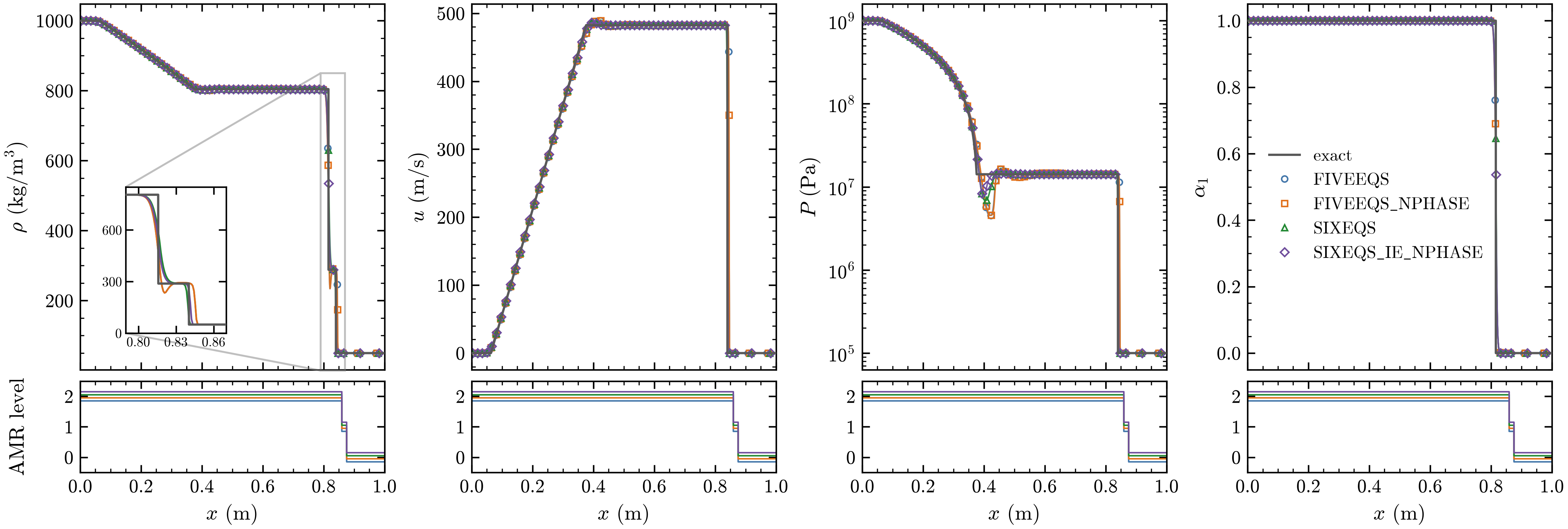
Water-air shock tube at \(t = 240\) µs with the four models and the exact solution for two stiffened gases (gray line): density \(\rho\), velocity \(u\), pressure \(P\) (log scale) and water volume fraction \(\alpha_1\). The inset enlarges the contact and the shock; the strips give the finest AMR level along \(x\).

The setup of Saurel and Abgrall (J. Comput. Phys. 150, 1999) puts water at 1000 kg/m\(^3\) and \(10^9\) Pa (stiffened gas, \(\gamma = 4.4\), \(P_\infty = 6 \times 10^8\) Pa) left of a diaphragm at \(x = 0.7\) m in a 1 m tube and air at 50 kg/m\(^3\) and \(10^5\) Pa to its right (\(\gamma = 1.4\)). The Sod case runs it through its prob.* parameters, with the grid and methods of Sod:

cd exec/_Tests/Sod && make -j4
mpirun -n 4 ./main3d.gnu.MPI.ex prob/inputs \
  stop_time=2.4e-4 amr.t_write_interval=2.4e-5 \
  prob.rho_L=1000 prob.P_L=1e9 prob.rho_R=50 prob.P_R=1e5 \
  prob.mat_R=2 prob.x_diaphragm=0.7 \
  prob.EOS.gamma_1=4.4 prob.EOS.pinf_1=6e8 \
  prob.EOS.gamma_2=1.4 prob.EOS.pinf_2=0.0

The other builds take the same keys with their inputs file, prob/inputs.Sod-6Eq and so on (the N-phase builds as arrays, prob.EOS.gamma="4.4 1.4" prob.EOS.pinf="6e8 0.0"). All four models reproduce the rarefaction into the water, the shock into the air and the plateaus, with pressure and velocity uniform across the contact. At the contact the six-equation models go from the water density to the shocked-air density directly, while the five-equation models dip slightly below it on the air side.

Noble-Abel stiffened gas

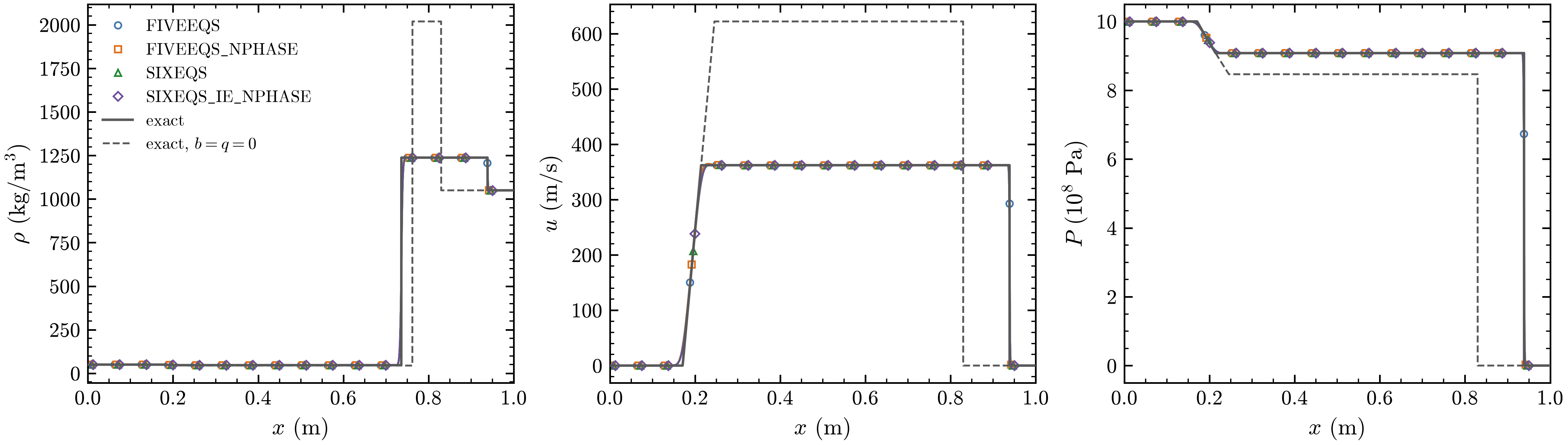
Air-water shock tube with liquid water as a Noble-Abel stiffened gas, at \(t = 0.1\) ms on 1024 cells, with the four models: density \(\rho\), velocity \(u\) and pressure \(P\) against the exact solution (gray line) and the exact solution for the same water without covolume and heat of formation, \(b = q = 0\) (gray dashed).

exec/_Tests/NASG runs the Noble-Abel stiffened gas with the four models (BUILD=5Eq, the default, 5Eq-N, 6Eq and 6Eq-N). Its inputs put air, an ideal gas, at 50 kg/m\(^3\) and \(10^9\) Pa left of a diaphragm at \(x = 0.7\) m in a 1 m tube, and liquid water at 1050 kg/m\(^3\) and \(10^5\) Pa to its right, with the parameters of Le Métayer and Saurel (Phys. Fluids 28, 2016): \(\gamma = 1.19\), \(P_\infty = 7.028 \times 10^8\) Pa, \(b = 6.61 \times 10^{-4}\) m\(^3\)/kg and \(q = -1.178 \times 10^6\) J/kg. The runs use MUSCL (minmod), HLLC and TVD-RK3; the six-equation inputs add the pressure relaxation. The figure has one level of 1024 cells:

cd exec/_Tests/NASG && make -j4
mpirun -n 4 ./main2d.gnu.MPI.ex prob/inputs amr.max_level=0 "amr.n_cell=1024 4" \
  amr.max_grid_size=128 amr.t_write_interval=1e-4

and the other models the same keys with their build and inputs file, for SIXEQS make -j4 BUILD=6Eq and ./main2d.gnu.MPI.6Eq.ex prob/inputs.NASG-6Eq. All four models follow the exact solution. The covolume matters: with \(b = q = 0\) the water is much softer, and the shock in the water lags far behind.

Shu-Osher problem

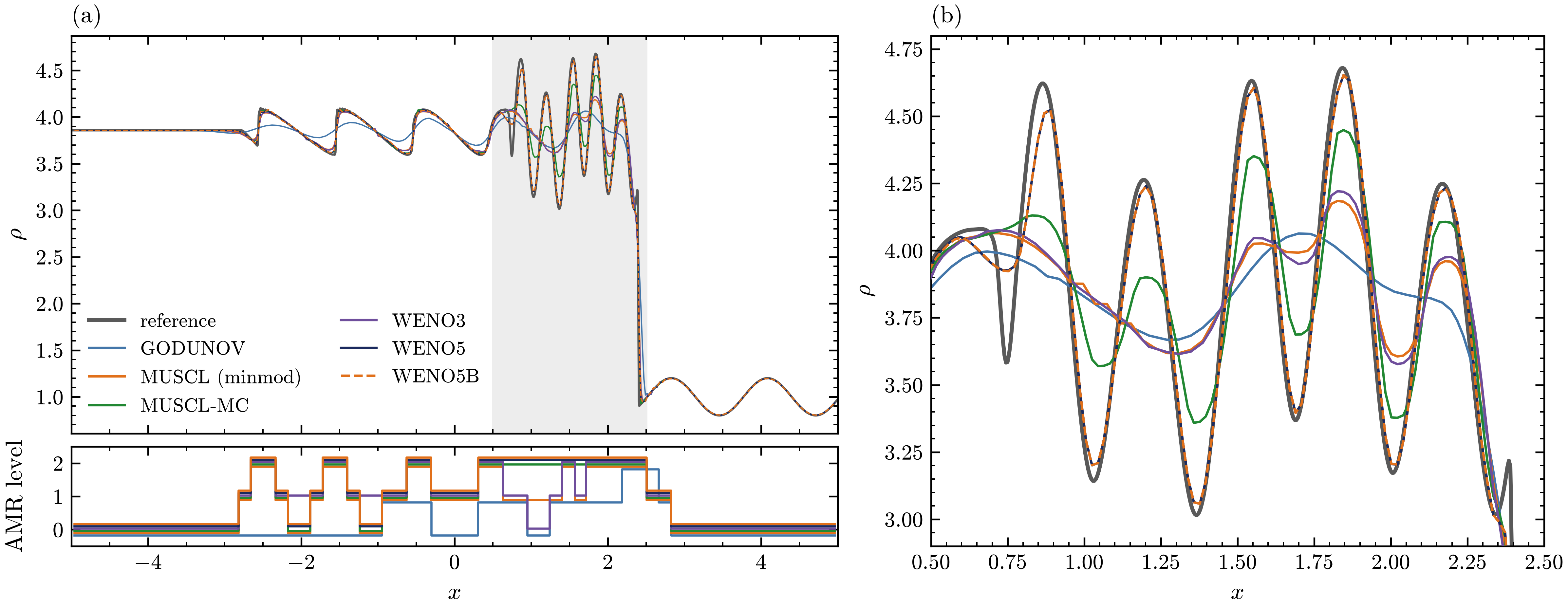
Shu-Osher problem: density at \(t = 1.8\) for each reconstruction scheme, against a WENO5 solution on 2048 cells (gray). (a) The whole tube, with the finest AMR level of each run below it. (b) The entropy waves behind the shock, the shaded region of (a). MUSCL uses the minmod limiter. WENO5B (dashed) lies on WENO5.

A Mach 3 shock at \(x = -4\) runs into the density perturbation \(\rho = 1 + 0.2\sin(5x)\) (Shu and Osher, J. Comput. Phys. 83, 1989). exec/_Tests/ShuOsher-5Eq runs it with a single fluid on 128 base cells with two levels of refinement, HLLC and TVD-RK3. The inputs use WENO5, and the other schemes are command-line overrides:

cd exec/_Tests/ShuOsher-5Eq && make -j4
mpirun -n 1 ./main2d.gnu.MPI.ex prob/inputs FiniteVolume.Scheme=MUSCL-MC

Godunov and MUSCL with minmod smear the entropy waves, MUSCL-MC and WENO3 recover part of their amplitude, and WENO5 and WENO5B follow the reference.

Planar water hammer

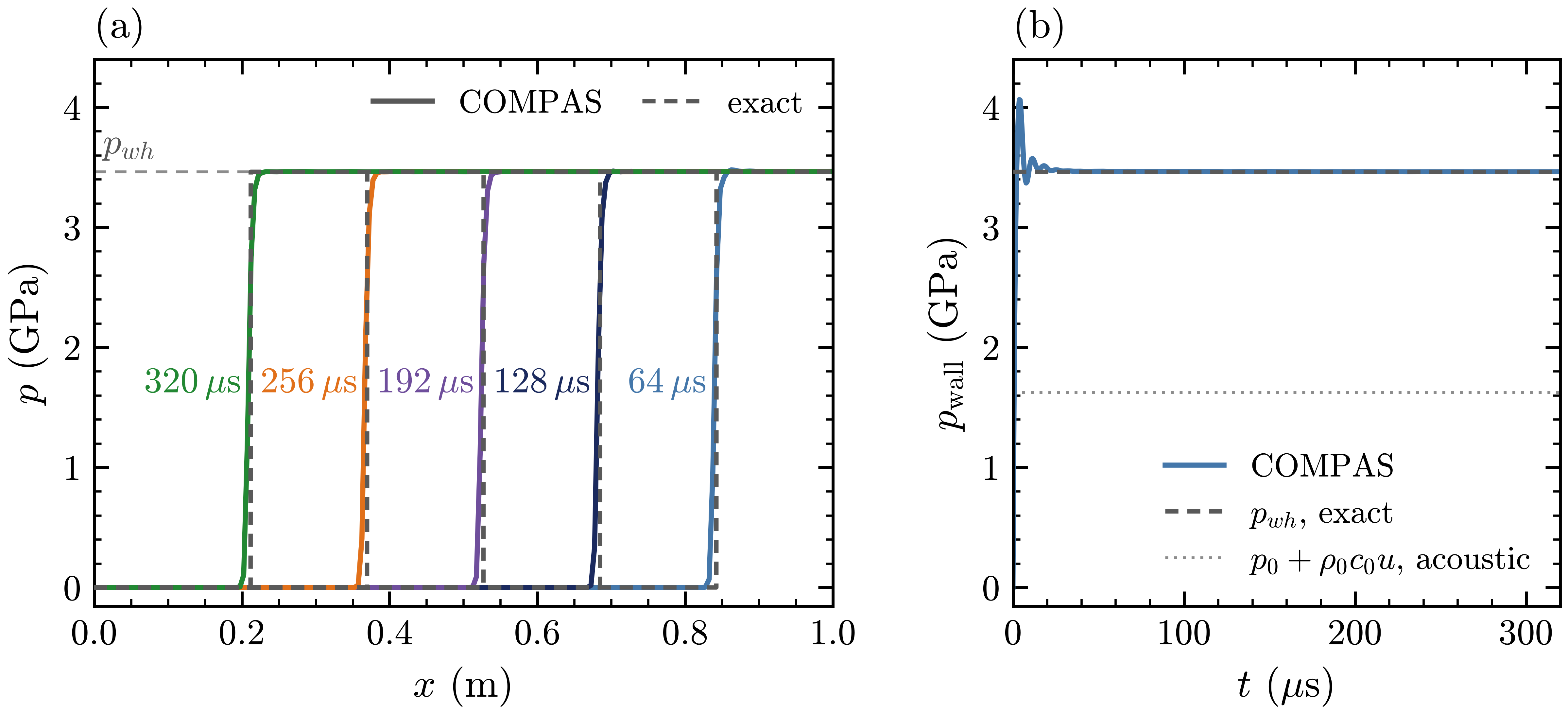
Planar water hammer with SIXEQS. (a) Pressure along the strip at 64, 128, 192, 256 and 320 µs, labeled at each shock, with the exact profiles (gray dashed) and the water-hammer pressure \(p_{wh}\). (b) Pressure at the wall against time, with the exact \(p_{wh}\) (gray dashed) and the acoustic estimate \(p_0 + \rho_0 c_0 u\) (dotted).

exec/WaterHammer-6Eq stops a column of water moving at \(u = 1000\) m/s against a slip wall. The water is a stiffened gas with \(\gamma = 4.4\) and \(p_\infty = 6 \times 10^8\) Pa, at \(\rho_0 = 1000\) kg/m\(^3\) and \(p_0 = 10^5\) Pa. Since \(p + p_\infty\) follows the ideal-gas Hugoniot and the wall is a piston in the frame of the incoming water, the shock runs back from the wall at \(W - u\), with

\[ W = \frac{\gamma+1}{4}\,u + \sqrt{\left(\frac{\gamma+1}{4}\,u\right)^2 + c_0^2}, \qquad p_{wh} = p_0 + \rho_0 W u, \qquad \rho_{wh} = \frac{\rho_0 W}{W - u}, \]

and \(c_0^2 = \gamma(p_0 + p_\infty)/\rho_0\): \(c_0 = 1625\) m/s, \(W = 3463\) m/s, \(p_{wh} = 3.46\) GPa and \(\rho_{wh} = 1406\) kg/m\(^3\), more than twice the acoustic estimate. The case uses pressure relaxation and air only as a trace, on a 1 m strip of 200 by 4 cells with MUSCL (minmod), HLLC and TVD-RK3, and runs to 320 µs in about a second:

cd exec/WaterHammer-6Eq && make -j3
mpirun -n 3 ./main2d.gnu.MPI.ex prob/inputs
python3 analysis/waterhammer.py plot/WaterHammer-6Eq

Parm::DynamicInit prints the exact solution, the case writes the shock position and the wall state to waterhammer.csv, and analysis/waterhammer.py compares them and draws the figure. The captured shock, spread over about three cells, runs back at the exact speed (within 0.03 percent after 80 µs) and stays within half a cell of the exact position. The plateau matches \(p_{wh}\) to within 0.01 percent, and the wall pressure settles within 0.1 percent of it after about 80 µs.

Shock reflection and convergence

Double Mach reflection

Double Mach reflection with WENO5, HLL, Δx = 1/480 on the finest of three AMR levels, from t = 0 to 0.2: 30 density contours from 1.73 to 21.5 over [0, 3] × [0, 1], and every patch box of levels 1 to 3 outlined in the color of its level. Download the MP4.

Woodward and Colella (J. Comput. Phys. 54, 1984) proposed the reflection of a Mach 10 shock in air off a 30 degree wedge as a test for shock-capturing schemes. exec/DoubleMachReflection-5Eq sets it up in the frame of the wedge on \([0, 4] \times [0, 1]\), with a single fluid and the boundary conditions restated by Kemm (Comput. Fluids 132, 2016): BoundaryFill_User fills the post-shock state on the left and ahead of the wedge, a mirror image along the wedge, and the exact moving shock on the top face. The base grid is 240 by 60 cells with three levels of refinement (\(\Delta x = 1/480\)) on the density jumps, MUSCL-MC, HLLC and TVD-RK3. The WENO5, HLL runs add the bound-preserving limiter and a blocking factor of 8, and the last one, with a plotfile every 0.0025, makes the video:

cd exec/DoubleMachReflection-5Eq && make -j4
mpirun -n 4 ./main2d.gnu.MPI.ex prob/inputs
mpirun -n 4 ./main2d.gnu.MPI.ex prob/inputs amr.max_level=2 amr.case_name=./plot/DoubleMach240
mpirun -n 4 ./main2d.gnu.MPI.ex prob/inputs FiniteVolume.Scheme=WENO5 Physics.RiemannSolver=HLL \
    FiniteVolume.ID_Bound=1 amr.blocking_factor_x="4 8" amr.blocking_factor_y="4 8" \
    amr.max_level=2 amr.case_name=./plot/DoubleMachWENO5_240
mpirun -n 4 ./main2d.gnu.MPI.ex prob/inputs FiniteVolume.Scheme=WENO5 Physics.RiemannSolver=HLL \
    FiniteVolume.ID_Bound=1 amr.blocking_factor_x="4 8" amr.blocking_factor_y="4 8" \
    amr.t_write_interval=0.0025 amr.case_name=./plot/DoubleMachWENO5
python3 analysis/triple_point.py plot/DoubleMach240 plot/DoubleMach \
    plot/DoubleMachWENO5_240 plot/DoubleMachWENO5 --figure dmr_zoom.png --ncols 2 \
    --labels 1/240 1/480 1/240 1/480 --row-labels "MUSCL-MC, HLLC" "WENO5, HLL"
python3 ../../scripts/postprocess.py movie plot/DoubleMachWENO5 --fps 10 --field none \
    --contour rho 1.73:21.5:30 --amr --amr-style boxes --amr-lw 0.6 --amr-alpha 0.7 --frame box \
    --xlim 0 3 --label '$t = {t:.3f}$' --width-px 2400 --out doublemach.mp4

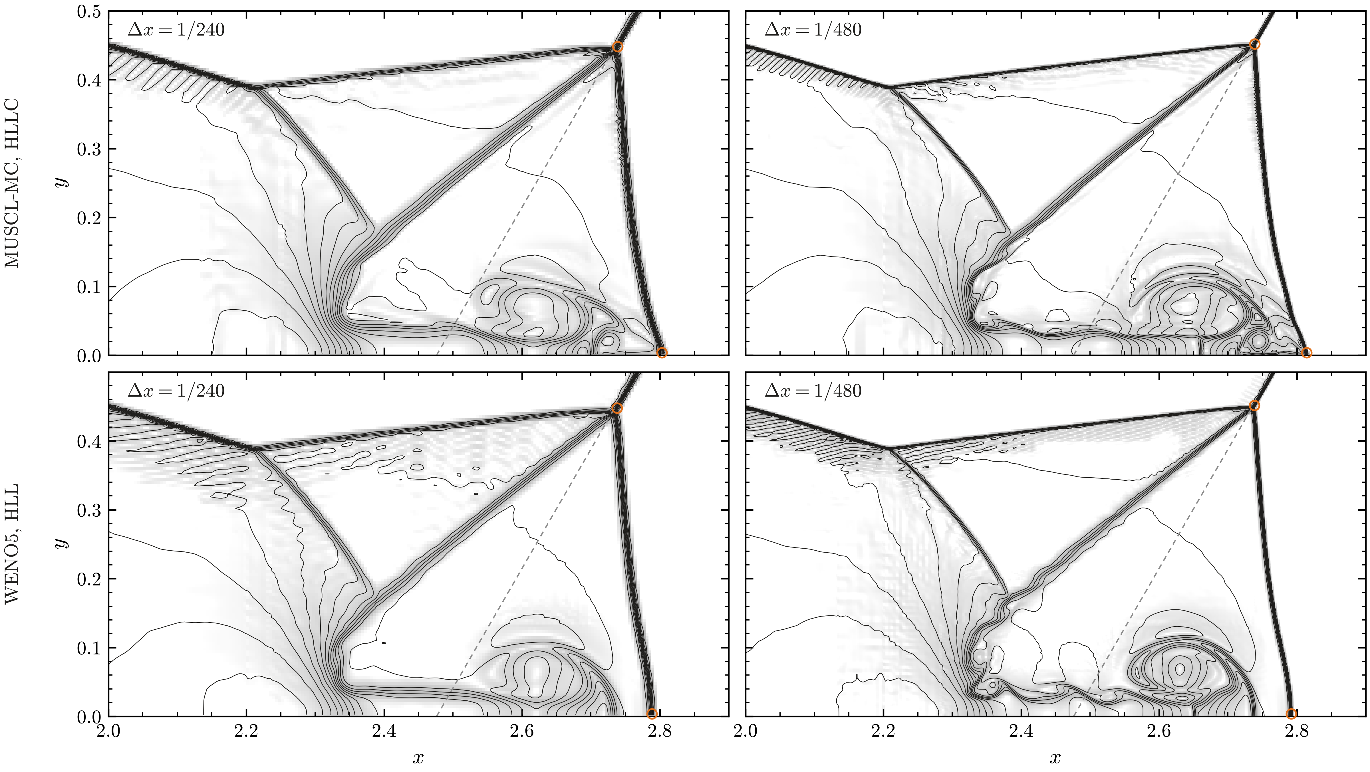
Close-up of \([2, 2.9] \times [0, 0.5]\) at \(t = 0.2\) with MUSCL-MC, HLLC (top row) and WENO5, HLL (bottom row), at \(\Delta x = 1/240\) (left) and \(1/480\) (right): density contours over a light density schlieren, which brings out the slip lines. Circles: the primary triple point and the foot of the Mach stem. Dashed line: the undisturbed incident shock.

Both schemes at both resolutions reproduce the structure of Woodward and Colella, from the Mach stem and the two triple points to the primary slip line, which turns forward along the wall into the jet. analysis/triple_point.py measures the primary triple point and the foot of the Mach stem and prints them next to three-shock theory. The triple point moves by less than two finest cells between the resolutions, its trajectory angle seen from the wedge tip is close to 10 degrees, and at \(\Delta x = 1/480\) the two schemes agree to within a fraction of a cell. With WENO5, HLL the Mach stem stands upright down to the wall and the slip line shows small roll-ups at \(1/480\). The foot of the Mach stem, written to stem.csv every coarse step, moves away from the wedge tip linearly in time, as in a self-similar reflection.

Guderley converging shock

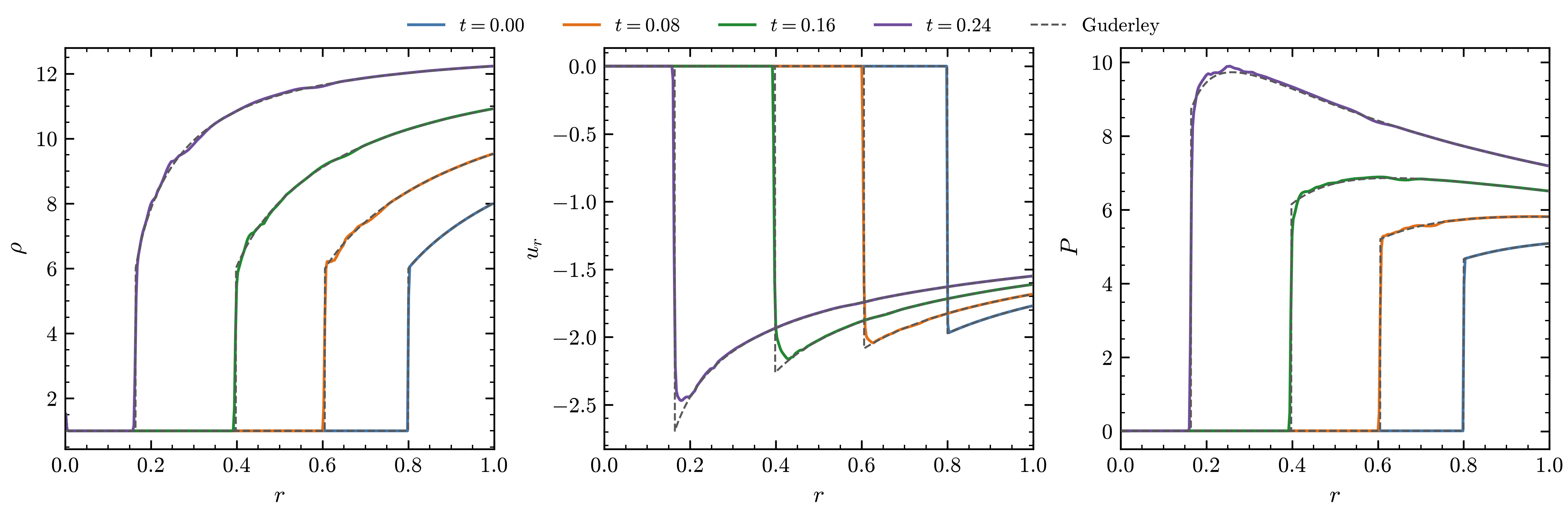
Guderley implosion with the interface removed (prob.R0=0 prob.a0=0): density \(\rho\), radial velocity \(u_r\) and pressure \(P\) along the \(x\) axis at \(t = 0\), 0.08, 0.16 and 0.24, against the similarity solution (gray dashed).

exec/GuderleyImplosion-5Eq is a strong cylindrical shock in air converging on a heavy gas; with the interface removed it is Guderley’s problem (1942). prob/Guderley.H finds the exponent of the shock trajectory \(R(t) = R_s (1 - t/\tau_c)^{\alpha}\) by bisection (\(\alpha = 0.835323\) for \(\gamma = 1.4\)) and tabulates the self-similar profile, which the case uses as the initial condition behind a Mach 20 shock at \(R_s = 0.8\) and, through BoundaryFill_User, as the exact inflow at the outer edges. One quarter of the plane is simulated on 96 by 96 base cells with two levels of refinement, MUSCL-MC and HLLC:

cd exec/GuderleyImplosion-5Eq && make -j4
mpirun -n 4 ./main2d.gnu.MPI.ex prob/inputs prob.R0=0 prob.a0=0 stop_time=0.25 amr.case_name=./plot/NoInterface
python3 analysis/plot_lineouts.py plot/NoInterface --times 0 0.08 0.16 0.24

The shock positions agree at every time shown and the profiles behind the shock follow the solution, with the velocity peak just behind the shock rounded off by the captured shock.

Order of accuracy

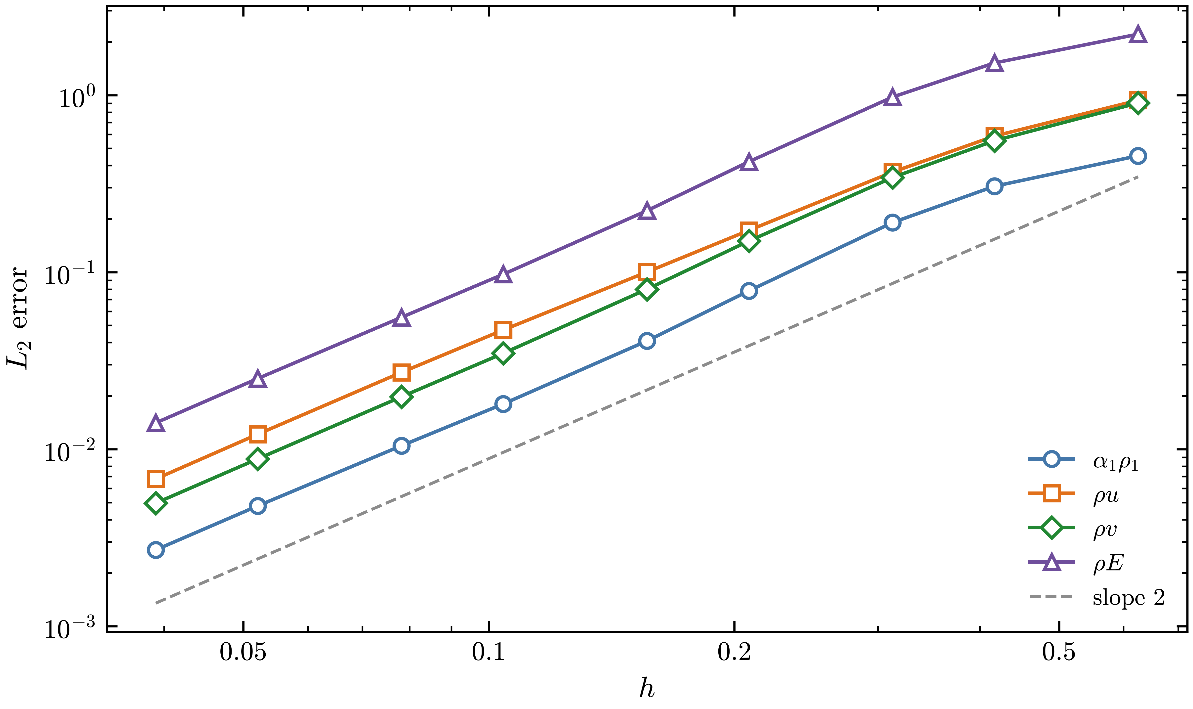
\(L_2\) error of the isentropic vortex with MUSCL-MC against the grid spacing \(h\), for \(\alpha_1\rho_1\), \(\rho u\), \(\rho v\) and \(\rho E\), on nine grids from 16 to 256 cells per side. The dashed gray line has slope 2.

exec/_Tests/IsentropicVortex-5Eq carries the isentropic vortex of Shu (1998) across the periodic box \([-5,5]^2\) for one period with WENO5. With CONVERGENCE defined in prob/ProblemICBC.H, COMPAS writes the error norms against the exact solution at the end of the run, and scripts/convergence.py runs the case over several resolutions and plots the errors. From the case directory,

python3 ../../../scripts/convergence.py --run --res 24 36 48 72 96
python3 ../../../scripts/convergence.py --vars a1rho1 rho_E rho_u --plot

The figure checks the second-order MUSCL scheme with the same case, switched to MUSCL-MC:

cp prob/inputs inputs_muscl
printf 'FiniteVolume.Scheme = "MUSCL-MC"\n' >> inputs_muscl
python3 ../../../scripts/convergence.py --run --inputs inputs_muscl --norm L2 --nprocs 3 --res 16 24 32 48 64 96 128 192 256
python3 ../../../scripts/convergence.py --vars a1rho1 rho_u rho_v rho_E --norm L2 --plot

The errors settle parallel to the slope-2 line as the grid is refined, the second-order accuracy expected of MUSCL-MC; on the coarsest grids, where the vortex spans few cells, they fall more slowly.

Viscous flows and heat conduction

The cases of this section are in exec/_Tests/Diffusion (-DDIFFUSION=true), one build per model: BUILD=5Eq, the default, for FIVEEQS, 6Eq for SIXEQS and 6Eq-N for SIXEQS_IE_NPHASE with two phases. prob.problem in each inputs file picks the problem.

Two-layer Couette flow

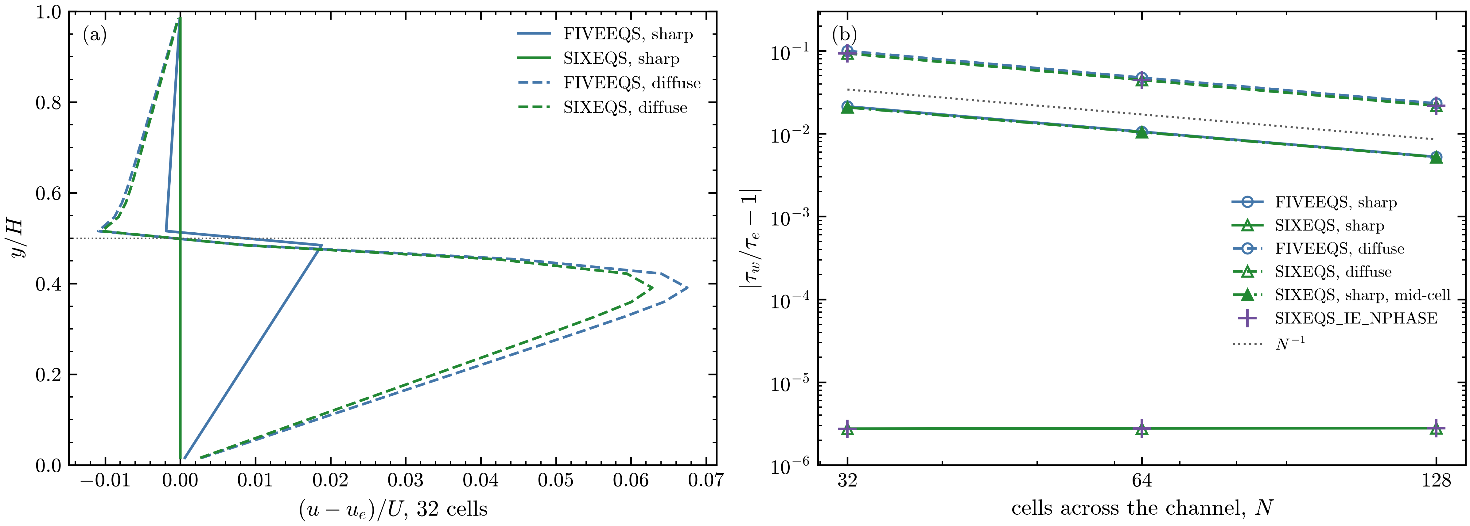
Two-layer Couette flow at \(t = 20\), viscosity ratio 10. (a) Departure of the velocity from the exact profile on 32 cells across the channel, with the interface on a cell face (sharp, solid lines) and as a tanh one cell wide (diffuse, dashed). (b) Error of the wall stress against the number of cells across the channel, also with the sharp interface in the middle of a cell (mid-cell), and for SIXEQS_IE_NPHASE (crosses). The dotted line has slope \(-1\).

Two layers at uniform pressure fill a channel between a wall at rest, \(y = 0\), and a wall moving at \(U = 0.01\), \(y = H = 1\): material 1, with \(\mu_1 = 0.01\) and \(\rho_1 = 1\), below \(y = h = H/2\), and material 2, with \(\mu_2 = 0.1\) and \(\rho_2 = 10\), above. The steady flow has a uniform shear stress and a velocity that is linear in each layer, with a kink at the interface:

\[\begin{split} \tau_e = \frac{U}{h/\mu_1 + (H - h)/\mu_2}, \qquad u_e(y) = \begin{cases} \tau_e\,y/\mu_1, & y < h,\\ \tau_e\left[h/\mu_1 + (y - h)/\mu_2\right], & y > h. \end{cases} \end{split}\]

The inputs start from this flow on a strip periodic in \(x\), 8 by 32 cells, and run to \(t = 20\) with MUSCL-MC, HLLC and TVD-RK3; the two walls are user boundary conditions. The case writes the wall stresses and their exact value to couette.csv every 20 coarse steps. "amr.n_cell=N/4 N" sets the grid, PhaseField.Eta_Multiplier=1 the diffuse interface and prob.h=(N/2 + 1/2)/N the interface in the middle of a cell, for example on 64 cells:

cd exec/_Tests/Diffusion && make -j4 && make -j4 BUILD=6Eq
mpirun -n 2 ./main2d.gnu.MPI.ex prob/inputs "amr.n_cell=16 64"
mpirun -n 2 ./main2d.gnu.MPI.6Eq.ex prob/inputs.Couette2Layer-6Eq "amr.n_cell=16 64"
mpirun -n 2 ./main2d.gnu.MPI.6Eq.ex prob/inputs.Couette2Layer-6Eq "amr.n_cell=16 64" \
  PhaseField.Eta_Multiplier=1 amr.case_name=./plot/Couette2Layer-6Eq-diffuse
mpirun -n 2 ./main2d.gnu.MPI.6Eq.ex prob/inputs.Couette2Layer-6Eq "amr.n_cell=16 64" \
  prob.h=0.5078125 amr.case_name=./plot/Couette2Layer-6Eq-midcell

Across the interface the traction is continuous and the velocity gradient jumps, so the two half cells next to a face act in series, and the harmonic mean of their viscosities, which the six-equation models use on the faces (Viscous and conductive fluxes in the six-equation models), is the exact face viscosity. With the interface on a face the profile is then exact. The arithmetic mean of the five-equation models overestimates the face viscosity at the interface and converges at first order. An interface inside a cell, or a diffuse interface, leaves mixed cells with the mixture viscosity, and both rules then converge at first order. SIXEQS_IE_NPHASE gives the SIXEQS results.

Conduction between two materials

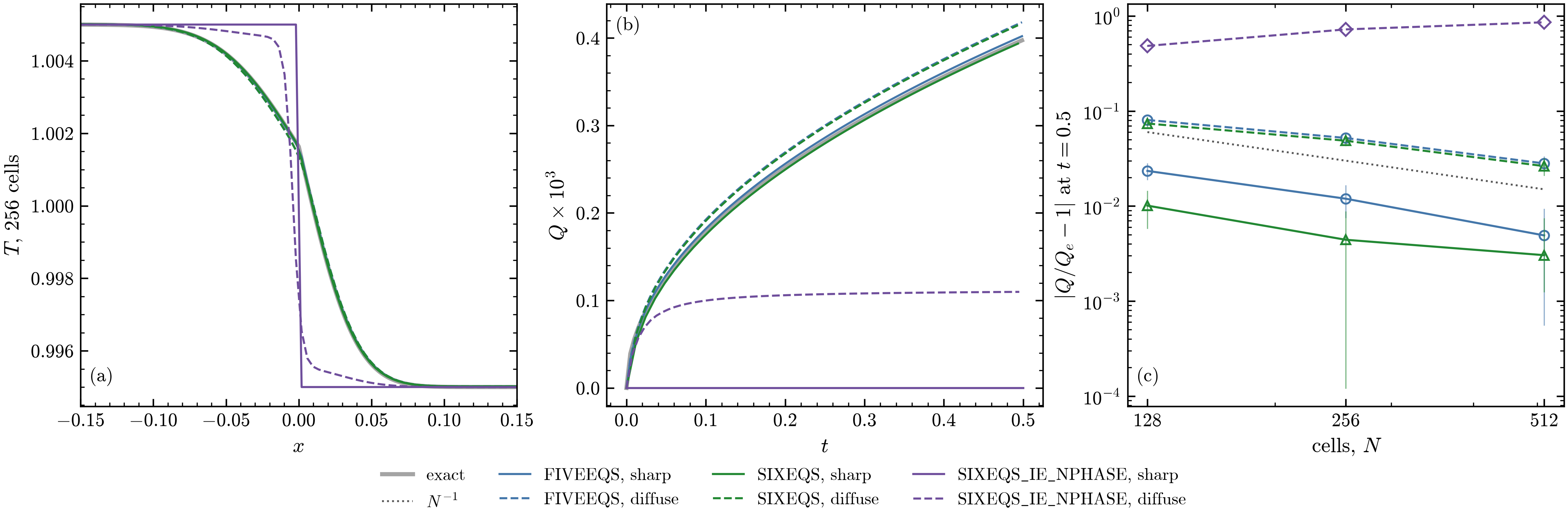
Heat conduction between two ideal gases. (a) Temperature at \(t = 0.5\) on 256 cells, with the interface on a cell face (sharp, solid lines) and as a tanh one cell wide (diffuse, dashed). (b) Heat \(Q\) through the interface against time. (c) Error of \(Q\) at \(t = 0.5\) against the number of cells: the line is the mean of the heat lost by \(x < 0\) and gained by \(x > 0\), the bar spans the two. Gray: the exact solution.

Two ideal gases at rest at the uniform pressure 1 meet at \(x = 0\): material 1 (\(\gamma = 1.4\), \(c_v = 2.5\), \(\kappa = 0.0063\)) at \(T_L = 1.005\) on the left and material 2 (\(\gamma = 5/3\), \(c_v = 0.375\), \(\kappa = 0.00225\), four times denser) at \(T_R = 0.995\) on the right. Between two semi-infinite media the interface takes at once the temperature

\[ T_i = \frac{e_L T_L + e_R T_R}{e_L + e_R}, \qquad e = \sqrt{\kappa\rho c_p}, \]

here \(T_i = 1.00163\), each side follows an erf profile with its own diffusivity, and the heat through the interface is \(Q_e = 2e_L(T_L - T_i)\sqrt{t/\pi}\). The inputs run it to \(t = 0.5\) on a strip of 256 by 8 cells, periodic in \(y\) and closed by adiabatic walls, with the interface one cell wide, and SIXEQS with the pressure-temperature relaxation. The case writes the heat through the interface, \(Q_e\) and the interface temperature to conduction.csv every 10 coarse steps. "amr.n_cell=N 8" sets the grid and PhaseField.Eta_Multiplier=0 the sharp interface:

cd exec/_Tests/Diffusion && make -j4 && make -j4 BUILD=6Eq && make -j4 BUILD=6Eq-N
mpirun -n 1 ./main2d.gnu.MPI.ex prob/inputs.HeatConduction2Mat-5Eq
mpirun -n 1 ./main2d.gnu.MPI.6Eq.ex prob/inputs.HeatConduction2Mat-6Eq
mpirun -n 1 ./main2d.gnu.MPI.6Eq-N.ex prob/inputs.HeatConduction2Mat-6Eq-N
mpirun -n 1 ./main2d.gnu.MPI.6Eq.ex prob/inputs.HeatConduction2Mat-6Eq PhaseField.Eta_Multiplier=0 \
  amr.case_name=./plot/HeatConduction2Mat-6Eq-sharp

In the five-equation models and in SIXEQS with the pressure-temperature relaxation the mixture conducts as one medium, and the temperature follows the two erf profiles. With the interface on a face the interface temperature and the heat converge to the exact values, closest with the harmonic mean of SIXEQS. With the diffuse interface the cells of the interface conduct with the mixture conductivity, and the error is first order in both. SIXEQS_IE_NPHASE has no temperature relaxation, so heat passes from one material to the other only through the mixed cells of a diffuse interface, and not through a sharp one (Viscous and conductive fluxes in the six-equation models).

Viscous shock tube

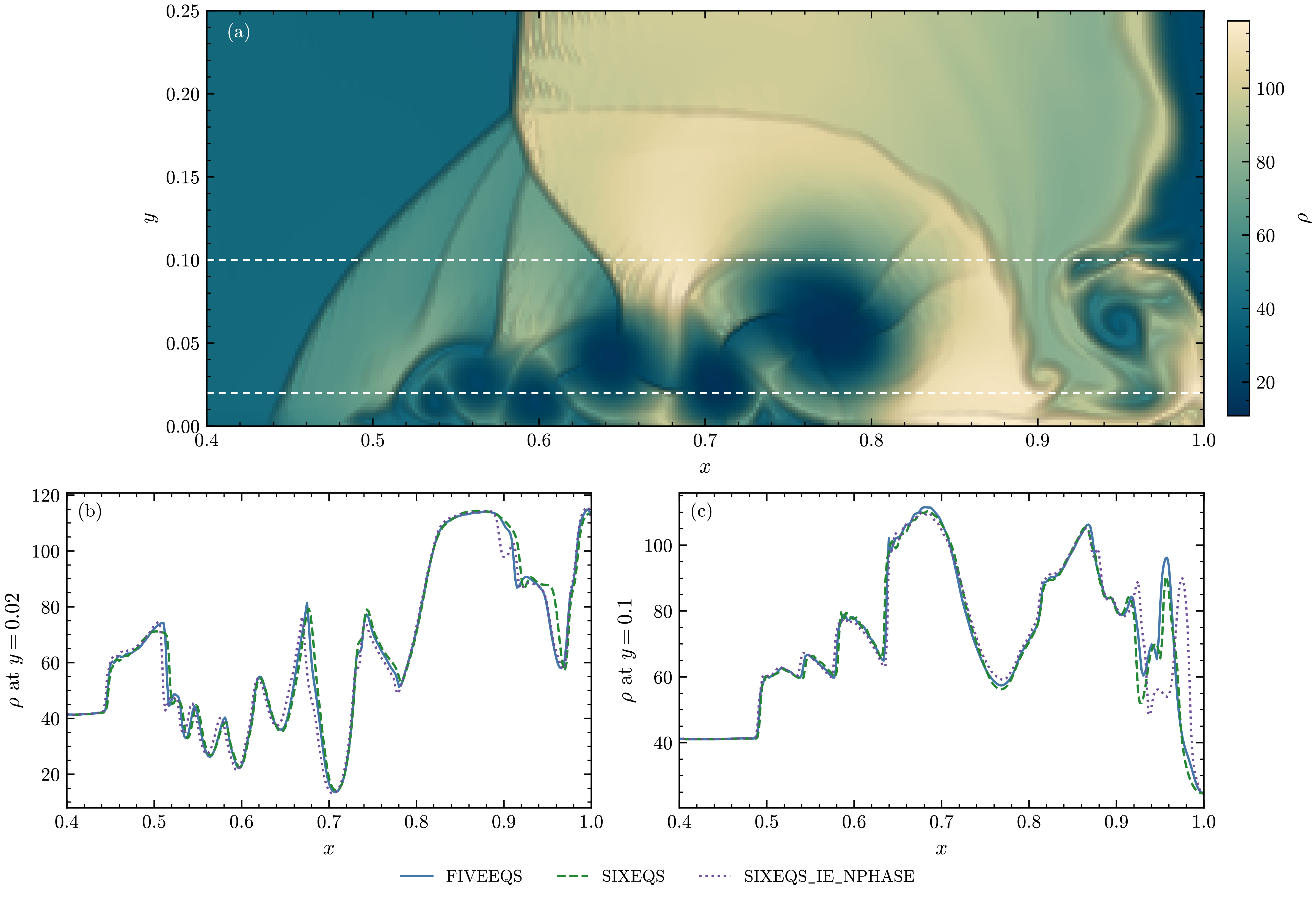
Viscous shock tube of Daru and Tenaud at \(Re = 1000\), \(t = 1\), on 512 by 256 finest cells. (a) Density of the FIVEEQS run near the right wall over the whole color map, from its smallest to its largest value, with a light schlieren on the steep gradients; the dashed lines are the lineouts. (b), (c) Density along \(y = 0.02\) and \(y = 0.1\) with the three models.

Daru and Tenaud (Comput. Fluids 38, 2009) proposed this test of a shock and a boundary layer: in a closed unit box with no-slip walls, a diaphragm at \(x = 0.5\) holds gas at rest with \(\rho = 120\), \(P = 120/\gamma\) against \(\rho = 1.2\), \(P = 1.2/\gamma\), \(\gamma = 1.4\), \(\mu = 1/Re\) and a Prandtl number of 0.73. The shock reflects from the right wall and meets the boundary layer it left on the bottom wall; the layer separates into vortices under a lambda shock. The lower half is simulated, with a slip wall at \(y = 0.5\). The test inputs (ViscousShockTube-5Eq, -6Eq, -6Eq-N) run it with one gas (in the six-equation models with a trace of \(10^{-6}\) of the other phase and the pressure relaxation) on 64 by 32 base cells with two levels of refinement, 256 by 128 at the finest, with WENO5, HLLC and TVD-RK3. The figure doubles the resolution:

cd exec/_Tests/Diffusion && make -j4 && make -j4 BUILD=6Eq && make -j4 BUILD=6Eq-N
mpirun -n 6 ./main2d.gnu.MPI.ex prob/inputs.ViscousShockTube-5Eq "amr.n_cell=128 64 8"
mpirun -n 6 ./main2d.gnu.MPI.6Eq.ex prob/inputs.ViscousShockTube-6Eq "amr.n_cell=128 64 8"
mpirun -n 6 ./main2d.gnu.MPI.6Eq-N.ex prob/inputs.ViscousShockTube-6Eq-N "amr.n_cell=128 64 8"

With one gas the models solve the same equations, and they give the same flow; the lineouts differ mostly in the vortex at the right wall.

Interface transport

Interface advection

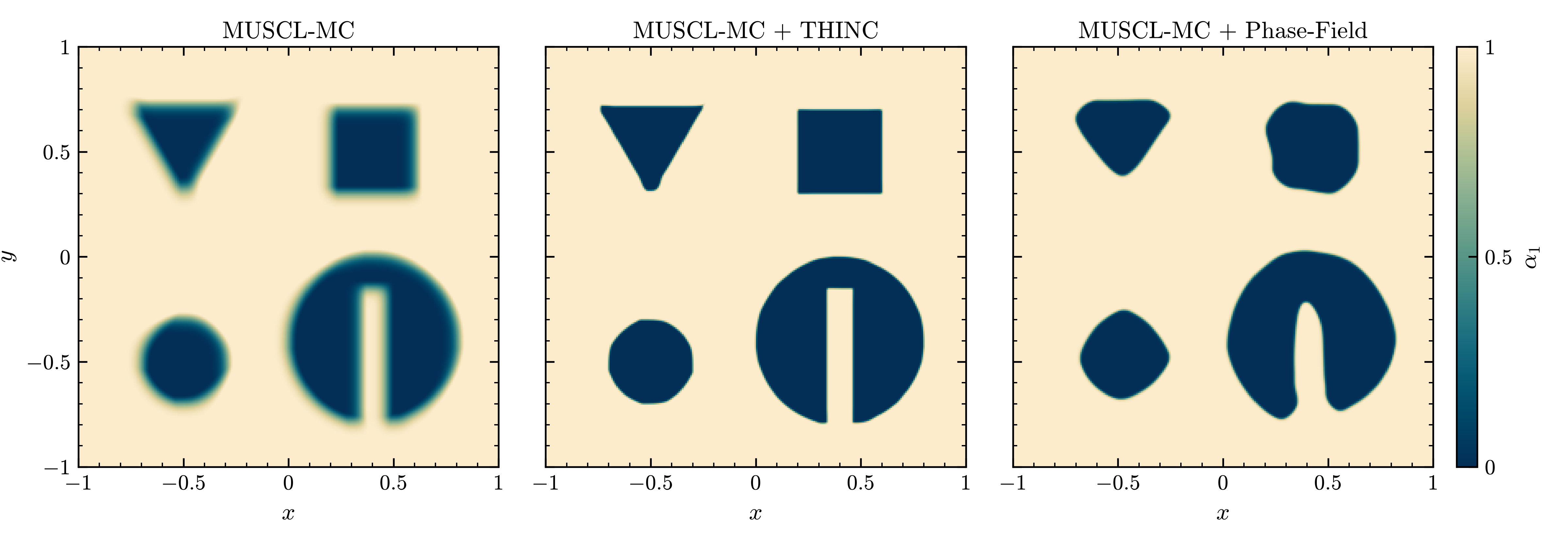
Volume fraction \(\alpha_1\) of the four shapes after one period (\(t = 2\)) with MUSCL-MC alone, MUSCL-MC + THINC and MUSCL-MC + Phase-Field (implicit CAC-Adv), each on 64 by 64 base cells with two levels of refinement.

The problem of the first simulation: a slotted disk (Zalesak, J. Comput. Phys. 31, 1979), a square, a circle and a triangle carried for one period across a periodic box at uniform pressure and velocity, so the exact solution is the initial condition. exec/_Tests/Advection runs the three with one executable, from prob/inputs (Advection-5Eq), prob/inputs.Advection-THINC-5Eq and prob/inputs.Advection-PF-5Eq, which differ only in the interface treatment.

MUSCL-MC alone spreads the interfaces over many cells, so that 14.8 % of the domain is mixed (\(0.05 < \alpha_1 < 0.95\)). THINC keeps the interfaces sharpest, with 2.5 % mixed, and the circle and the slotted disk nearly round; only the lower corner of the triangle ends in a small rounded knob. The one-dimensional THINC (Numerics) turns the circle into an octagon, with 2.3 times the error. Phase-Field holds the interfaces at a fixed width (3.4 % mixed), but at this resolution, with \(\eta\) half a finest cell, it also reshapes them: the corners round off, the circle becomes a rounded diamond and the slot partly closes.

Vortex windup

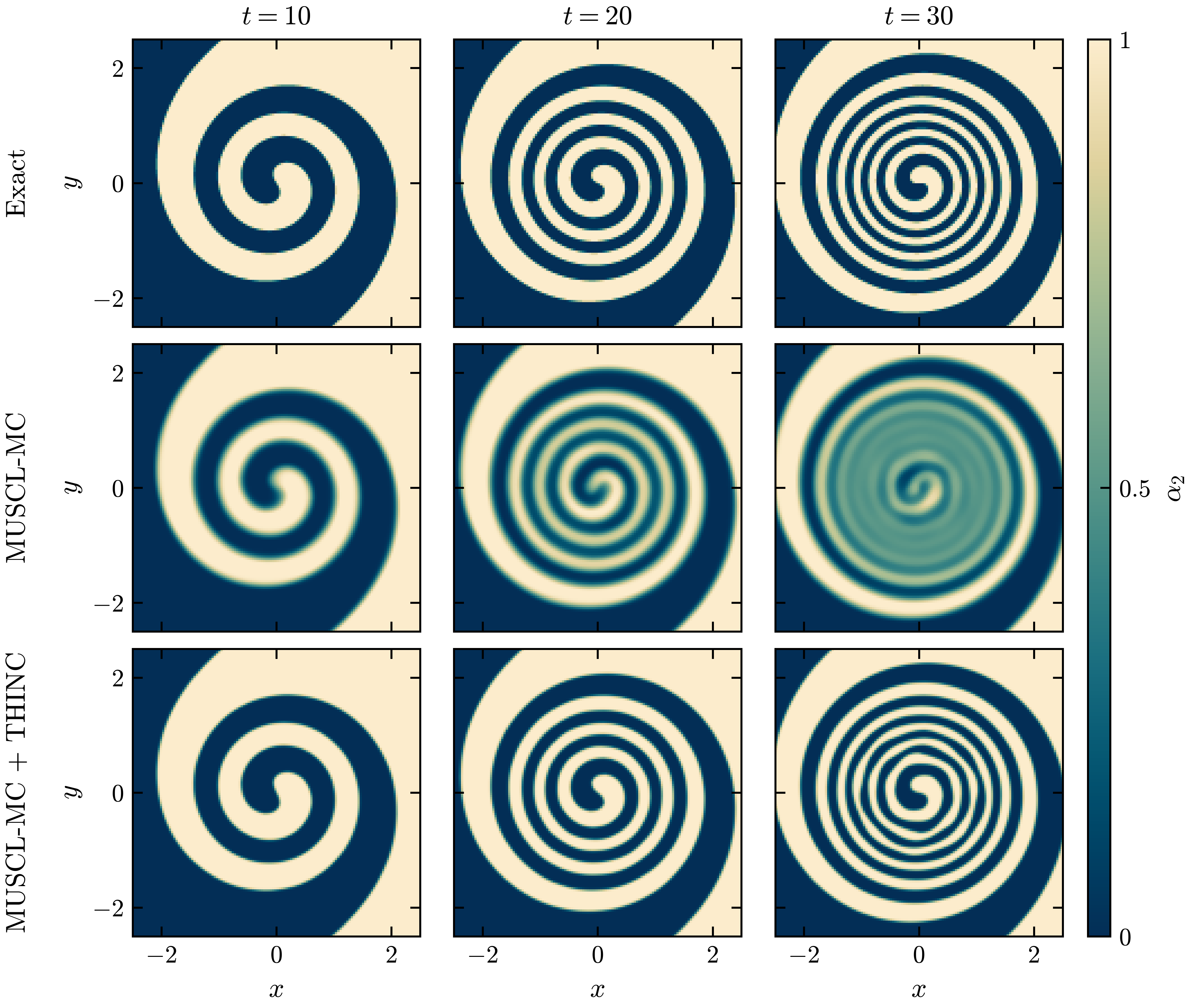
exec/VortexWindup-5Eq at \(t = 10\), 20 and 30, when the center has turned 2.1, 4.2 and 6.3 times: the exact volume fraction \(\alpha_2\) of material 2 (top row), MUSCL-MC alone (middle row) and MUSCL-MC + THINC (bottom row), in \(|x|, |y| < 2.5\). Material 1 dark blue, material 2 sand.

exec/VortexWindup-5Eq winds a straight interface through the center of a steady isentropic vortex (Shu, 1998) of strength \(\beta = 5\) and core radius \(r_c = 1\) into a double spiral, in the box \([-5, 5]^2\). Both materials are the same gas at the same density, so the interface is passive: each point turns at \(\Omega(r) = \beta/(2\pi r_c)\, e^{(1 - r^2/r_c^2)/2}\), and the exact volume fraction is the initial one turned by \(-\Omega(r)\,t\). The arms thin in time, the thinnest, near \(r = r_c\), being about \(4/t\) wide, so the case tests how long a scheme keeps a sharp interface whole in a sheared flow. The inputs run to \(t = 30\), when these arms are 3.4 cells wide, on 256 by 256 cells with MUSCL-MC, HLLC, TVD-RK3 and THINC:

cd exec/VortexWindup-5Eq && make -j4
mpirun -n 2 ./main2d.gnu.MPI.ex prob/inputs
mpirun -n 2 ./main2d.gnu.MPI.ex prob/inputs FiniteVolume.THINC=0 amr.case_name=./plot/VortexWindup-MUSCL
python3 analysis/windup.py plot/VortexWindup-MUSCL plot/VortexWindup --labels MUSCL-MC THINC \
    --csv windup_metrics.csv --plot windup.png --time 30

The case writes the volume of material 2, the bounds of \(\alpha_1\), the mixed area and the \(L_1\) error to windup.csv, and analysis/windup.py computes the error and the number of pieces the arms break into from the plotfiles.

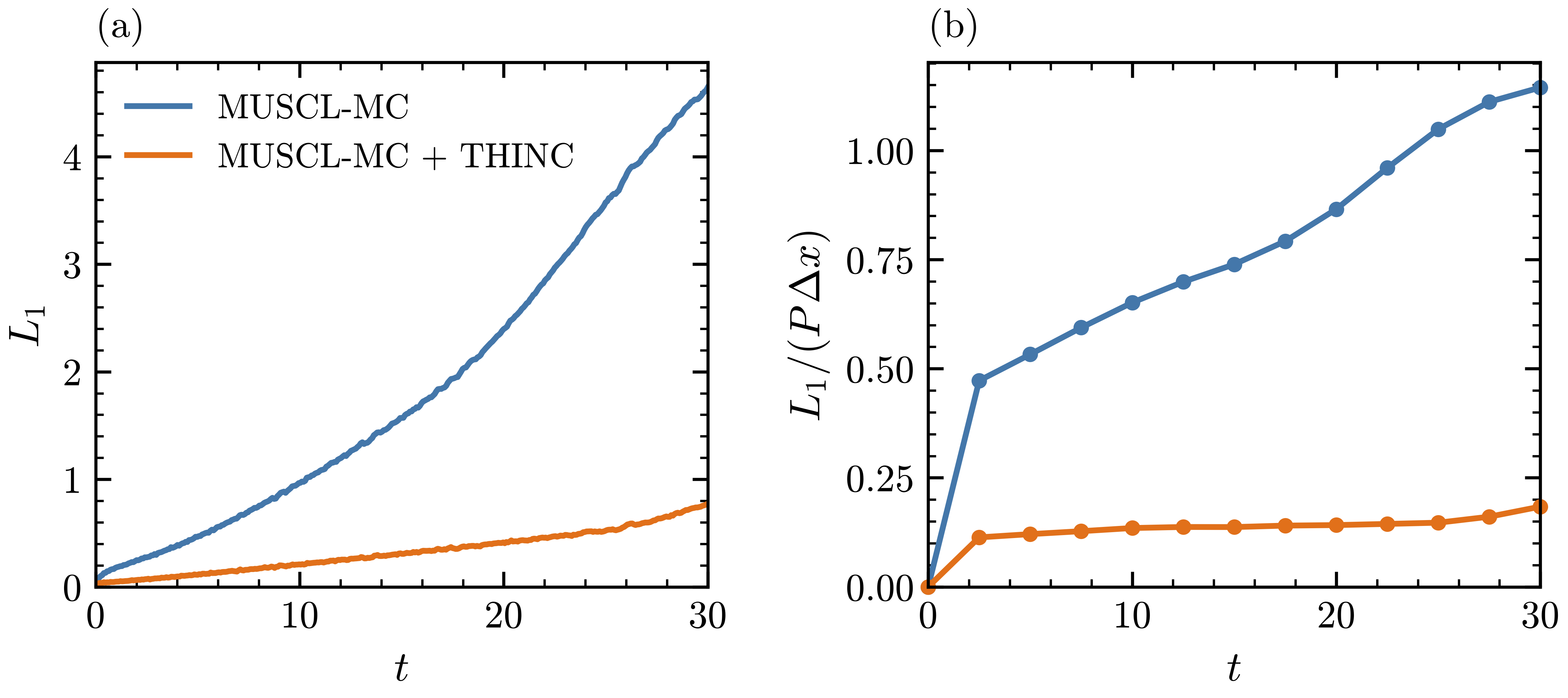
(a) \(L_1 = \int |\alpha_2 - \alpha_{2,\mathrm{exact}}|\,\mathrm{d}A\) of the two runs, from windup.csv. (b) \(L_1/(P\,\Delta x)\), the mean width of the error in cells, with \(P\) the length of the exact interface.

MUSCL-MC spreads the interface over four to five cells, and once the arms are thinner than that the inner turns blend together: by \(t = 30\) they have merged into a region of \(\alpha_2 \approx 0.5\), split into four extra pieces, and \(L_1 = 4.6\). With THINC the interface stays about two cells wide, the mean width of the error stays between 0.11 and 0.15 cells until \(t = 25\), and the spiral is whole at \(t = 30\), with \(L_1 = 0.74\), a sixth of the MUSCL-MC error. The volume of material 2 is kept to two parts in \(10^7\). The one-dimensional THINC breaks the inner arms into beads by \(t = 27.5\) and ends with six extra pieces and \(L_1 = 1.6\).

Shock-interface interaction

Shock through two interfaces

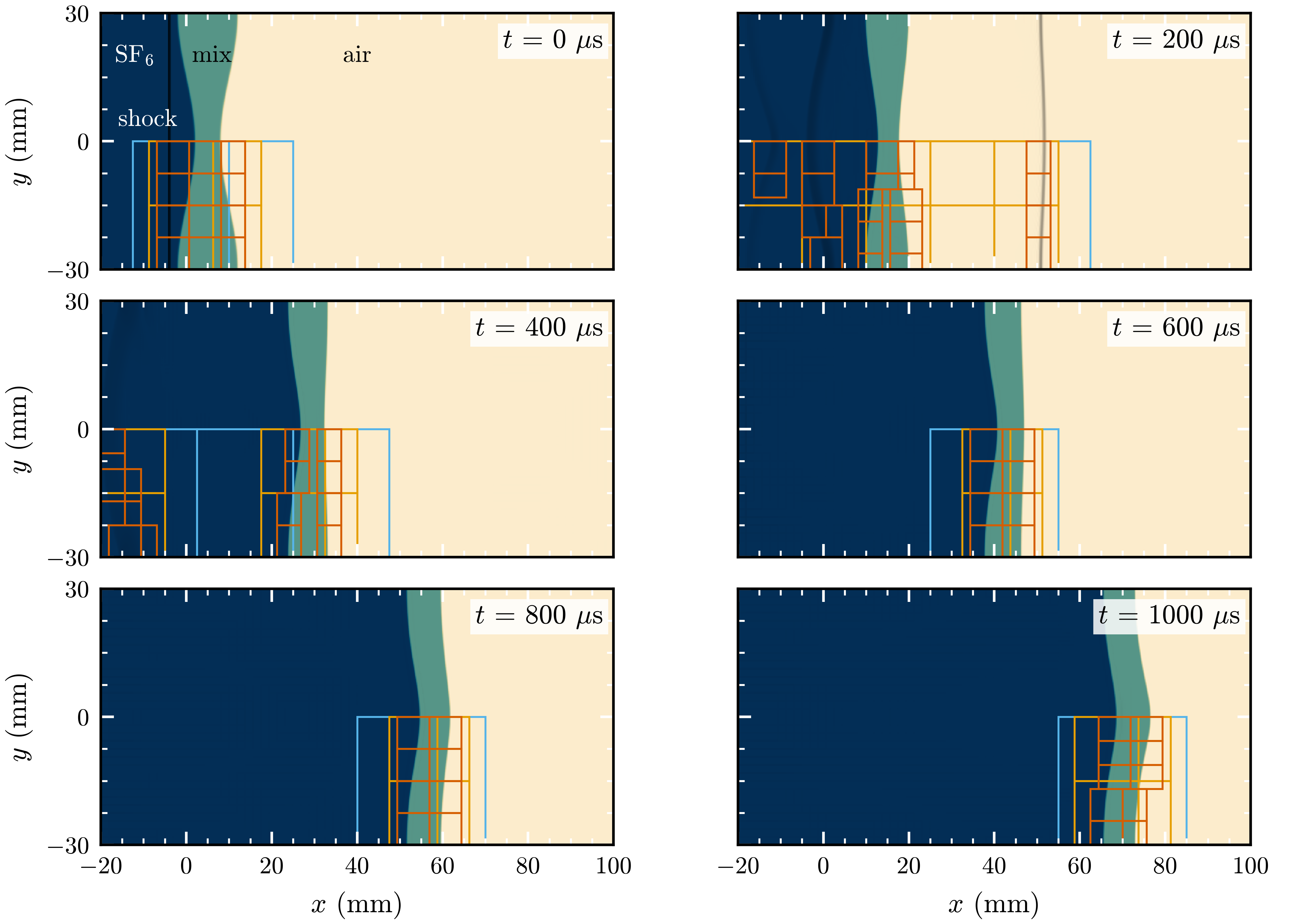
exec/ThreeMaterialRM-5Eq-N with perturbed interfaces and THINC, three levels of refinement, from \(t = 0\) to 1000 µs, mirrored about \(y = 0\) to show a full wavelength: SF\(_6\) dark blue, mixture teal and air sand, blended by volume fraction. A numerical schlieren darkens the shocks in pure fluid more than three cells from any interface. Lower half: AMR patches of levels 1 (light blue), 2 (orange) and 3 (vermilion).

exec/ThreeMaterialRM-5Eq-N reproduces the shock-tube experiments of Liang and Luo (J. Fluid Mech. 955, 2023), as in section 4.3 of the COMPAS paper. A Mach 1.24 shock in SF\(_6\) (material 1) crosses a 10 mm layer of an SF\(_6\)-air mixture (material 2) into air (material 3). Both interfaces carry a 2 mm sinusoidal perturbation of wavelength 60 mm, in anti-phase. Half a wavelength is simulated with ideal gases in SI units, on 80 by 16 base cells with three levels of refinement, MUSCL-MC and HLLC (the paper uses five levels). The case writes the interface positions, the amplitudes and the thickness of material 2 to interfaces.csv every coarse step, and analysis/plot_interfaces.py plots them. The perturbed and flat runs, with MUSCL-MC alone and with THINC, are

cd exec/ThreeMaterialRM-5Eq-N && make -j4
mpirun -n 4 ./main2d.gnu.MPI.ex prob/inputs
mpirun -n 4 ./main2d.gnu.MPI.ex prob/inputs prob.amp=0 amr.case_name=./plot/Flat
mpirun -n 4 ./main2d.gnu.MPI.ex prob/inputs FiniteVolume.THINC=1 amr.case_name=./plot/THINC
mpirun -n 4 ./main2d.gnu.MPI.ex prob/inputs FiniteVolume.THINC=1 prob.amp=0 amr.case_name=./plot/FlatTHINC

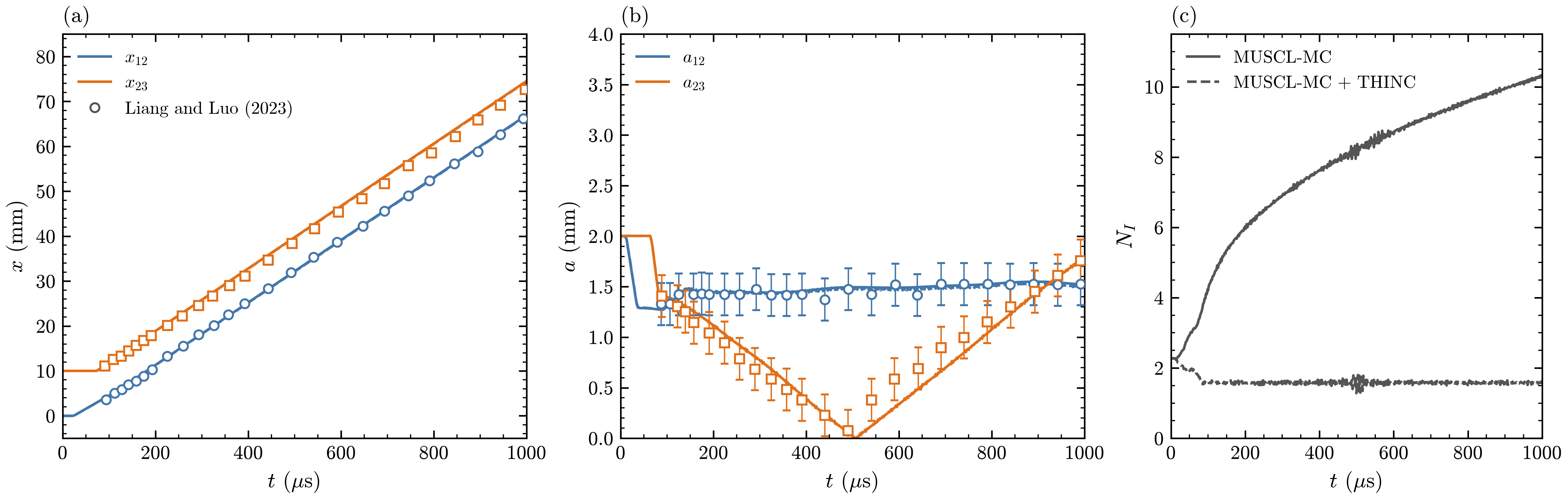
Against the measurements of Liang and Luo (2023): circles for the first interface, squares for the second, with the measurement times shifted by 24 µs, the time the simulated shock takes to reach the first interface. (a) Flat interfaces: positions \(x_{12}\) and \(x_{23}\). (b) Perturbed interfaces (\(a_0 = 2\) mm, \(\lambda = 60\) mm): amplitudes \(a_{12}\) and \(a_{23}\), with the 0.208 mm error bar of the measurements. (c) Perturbed run: thickness \(N_I\) of the material-2 interface, in cells. Solid lines: MUSCL-MC; dashed lines: MUSCL-MC + THINC.

The positions of both flat interfaces follow the measurements over the whole run. The first perturbed interface is compressed by the shock and then nearly frozen by the rarefaction reflected from the second, as in the experiment. The amplitude of the second interface falls, passes through zero close to the measured time as the interface inverts, and grows with the opposite phase; it is within the error bars before the inversion and near the end of the run. With THINC the thickness of material 2 stays between 1.3 and 1.8 cells from 80 µs to the end, against 10.3 cells at 1000 µs with MUSCL-MC alone, while the amplitudes and positions stay within 0.04 and 0.12 mm of the MUSCL-MC run: the waves set them, and the interface width hardly changes them.

Shock and helium cylinder

The run from shock arrival to 1 ms, with the quantities of the x-t diagram below marked at the time of each frame. Left: air white and helium wine, and in the mirrored lower half the pressure schlieren, the interface and the outlines of AMR levels 1 to 5, in a window that follows the helium. On the axis, the circle is the upstream interface and then the jet head, and the square the downstream interface, where the helium volume fraction crosses 0.5; the triangle is the upstream extreme of the helium and, from 400 µs, the cross the centroid of the vortex pair. Until 115 µs the arrowheads mark the incident shock (on the row y = 40 mm, drawn in the schlieren half) and the refracted, then transmitted, wave. Right: the x-t diagram, each line drawn up to the time of the frame, with the points of Haas and Sturtevant appearing as they are passed. Download the MP4.

Haas and Sturtevant (J. Fluid Mech. 181, 1987) photographed a Mach 1.22 shock in air passing over a 5 cm helium cylinder held by a thin plastic membrane. exec/ShockBubble-AirHelium-5Eq sets up the problem in nondimensional units, with cylinder radius 0.25, the air ahead of the shock at pressure 1 and density 1.2, and the upper half simulated. The helium held an air mass fraction of 0.28 (the paper’s estimate), which gives a density ratio of 0.182 to the air and, mixing the two ideal gases by mole fraction, \(\gamma = 1.645\). The run uses these values, MUSCL-MC with THINC and five levels of refinement, 256 finest cells per radius, with plotfiles at the times of the photographs, every 0.01 while the waves cross the cylinder and every 0.04 after:

cd exec/ShockBubble-AirHelium-5Eq && make -j4
mpirun -n 4 ./main2d.gnu.MPI.ex prob/inputs FiniteVolume.Scheme=MUSCL-MC FiniteVolume.THINC=1 \
    prob.Mach=1.22 prob.rho2=0.2186 prob.EOS.gamma_2=1.645 amr.max_level=5 stop_time=3.2 \
    amr.t_write="0.12089 0.18458 0.21643 0.24828 0.28013 0.34382 0.79925 1.37889 2.16554 3.14965" \
    amr.n_output_windows=1 amr.output_window_0.t_lo=0 amr.output_window_0.t_hi=0.6 \
    amr.output_window_0.dt=0.01 amr.t_write_interval=0.04 \
    run.output_vars="a1 rho u v P" amr.case_name=./plot/HS

Lengths are scaled with the radius (0.25 for 25 mm) and velocities with the sound speed of the air (\(\sqrt{1.4/1.2}\) for 344 m/s), so one time unit is 314 µs. The shock starts \(0.1R\) upstream of the cylinder, and time is counted from its arrival there, as in the paper.

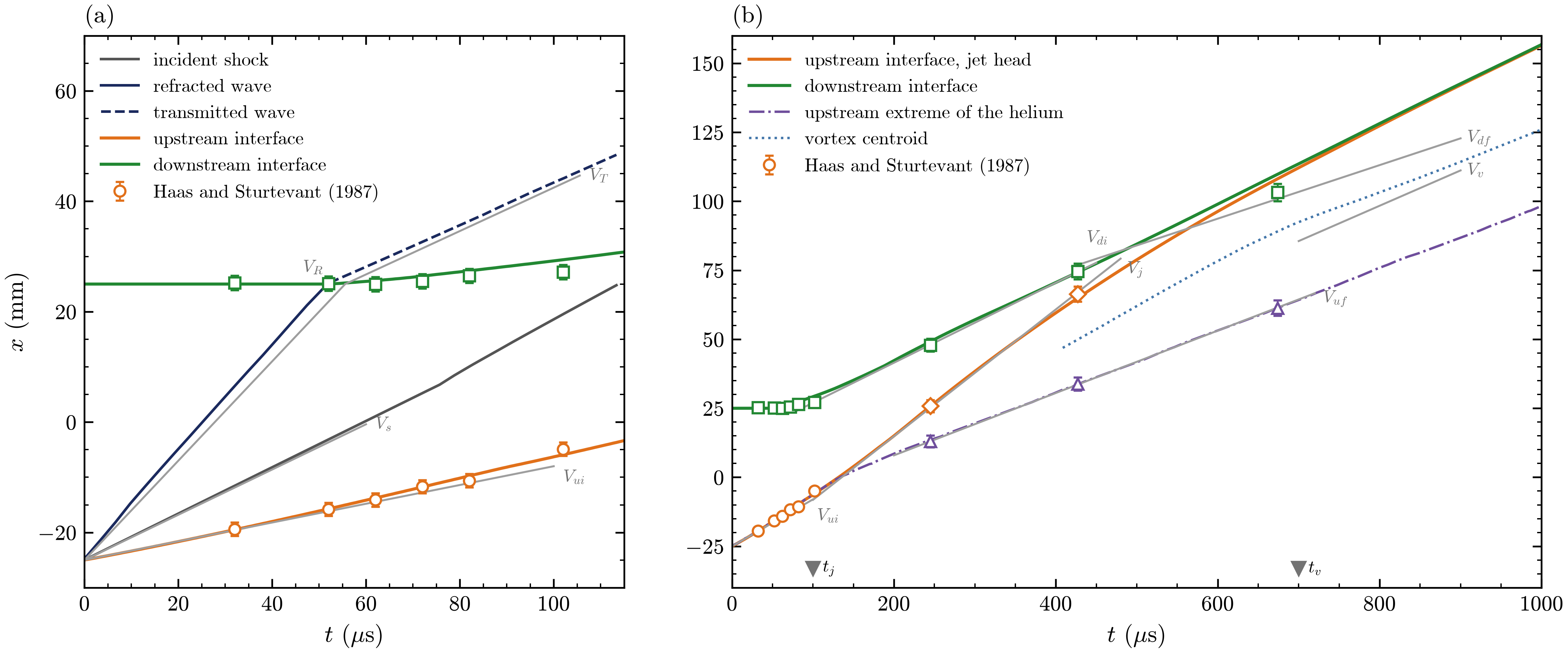
\(x\)-\(t\) diagram of the interaction against the shadowgraphs of Haas and Sturtevant (1987, Fig. 7), with the symbols colored like the lines they measure; \(t\) from the arrival of the shock at the cylinder and \(x\) from the initial cylinder axis. (a) Early times: the incident shock outside the cylinder (row \(y = 40\) mm); the refracted wave on the axis, dashed once it leaves the helium as the transmitted wave; the upstream and downstream interfaces on the axis. (b) The whole run: the upstream interface on the axis and then the jet head; the downstream interface on the axis; the upstream extreme of the helium; the centroid of the vortex pair (from 400 µs). Short gray lines: the velocities of their Table 2. Triangles: their jet and vortex formation times.

The interfaces on the axis come from bubble.csv, written every coarse step, and the other lines from the plotfiles. The refracted wave runs through the helium at 953 m/s (900 m/s in Table 2) and leaves it after about 52 µs as the transmitted wave, at 380 m/s (393 m/s). The upstream interface passes within 1 mm of the measured points and accelerates into the re-entrant air jet, whose head crosses the helium at 226 m/s (230 m/s). The upstream extreme of the helium follows the measured points to within 1 mm, at 112 m/s (113 m/s) late in the run, and the downstream interface follows them to within 2.2 mm up to 427 µs. The vortex pair travels at 111 m/s, slower than the measured 128 m/s. Once the jet reaches the downstream interface, the photographs show it spreading along that interface, while in the simulation it pushes the thin helium layer on the axis ahead of it, so the downstream point leads the measurements, by 6.6 mm at 674 µs. The simulated lobes roll up into tight spirals where the photographs show broad, finely mixed lobes, and from about 245 µs short waves about 20 finest cells long roll up along the sheared outer edge of each lobe.

Shock refraction at an air-water interface

The four runs, each until the refraction point reaches y = 32 mm, with the measurements of analysis/refraction.py applied to every frame: air volume fraction (sand air, teal water) darkened by a light pressure schlieren, and the patch boxes of AMR levels 1 and 2 at β = 50°. The white circle is the refraction point. The wave angles are measured on arcs around it (every fourth arc is drawn), at the points where the pressure crosses halfway across each shock (dots): the magenta line is the direction fitted to the dots and the dashed line that of polar theory. The orange triangle is the leading edge of the precursor, where the wall pressure has risen by 1 percent of the jump across the incident shock. At 50° the reflected shock is followed in columns just behind the incident shock (zoom), and the line through it meets the incident shock at the triple point (diamond), drawn with its track. Download the MP4.

Anbu Serene Raj, Vishnu Prasad, Rajesh and Sameen (J. Fluid Mech. 998, A49, 2024) photographed a Mach 1.46 shock in air refracting at the inclined surface of water, and explained the patterns with shock polars for a stiffened gas. The pattern depends on the angle \(\beta\) between the shock and the interface, along which the refraction point runs at \(U_s/\sin\beta\). While this speed exceeds the sound speed of the water, \(c_w = 1503\) m/s, the incident, reflected and transmitted shocks meet at the refraction point (regular refraction, RRR). Below it, at \(\beta = 19.7^\circ\) for this shock, the transmitted wave runs ahead as a free precursor, under a regular reflection in the air (FPR) or, once that reflection detaches, a Mach reflection (FMR).

exec/ShockRefraction-AirWater-5Eq uses the paper’s values: air an ideal gas with \(\gamma = 1.4\), water a stiffened gas with \(\gamma = 2.8\), \(P_\infty = 8.5 \times 10^8\) Pa and \(\rho = 1053\) kg/m\(^3\), both at rest at 101325 Pa, in a 100 by 40 mm domain. The water fills a wedge with its apex on the bottom slip wall and its surface at \(90^\circ - \beta\) to the wall (prob.beta), and the left boundary feeds in the state behind the shock. As in the paper, the volume fraction is advected without the \(K \nabla \cdot \mathbf{u}\) term, and the interface starts sharp. The runs use MUSCL (van Leer), HLLC, TVD-RK3 and THINC, on 200 by 80 base cells of 0.5 mm with two levels on the interface and the pressure gradient, and each stops when the refraction point reaches \(y = 32\) mm:

cd exec/ShockRefraction-AirWater-5Eq && make -j4
mpirun -n 3 ./main2d.gnu.MPI.ex prob/inputs prob.beta=15   stop_time=20.9e-6 amr.case_name=./plot/b15/plot
mpirun -n 3 ./main2d.gnu.MPI.ex prob/inputs prob.beta=20.5 stop_time=27.6e-6 amr.case_name=./plot/b20.5/plot
mpirun -n 3 ./main2d.gnu.MPI.ex prob/inputs prob.beta=30   stop_time=40.4e-6 amr.case_name=./plot/b30/plot
mpirun -n 3 ./main2d.gnu.MPI.ex prob/inputs prob.beta=50   stop_time=79.2e-6 amr.case_name=./plot/b50/plot
python3 analysis/polar.py
python3 analysis/refraction.py waves plot --out shockrefraction_waves.png

The case writes the incident shock, the refraction point and the front of the transmitted wave along the wall to waves.csv every coarse step. analysis/polar.py solves the stiffened-gas oblique-shock relations of the paper, and analysis/refraction.py waves measures the wave angles, the precursor and the triple point, as the video shows, and draws the figure below.

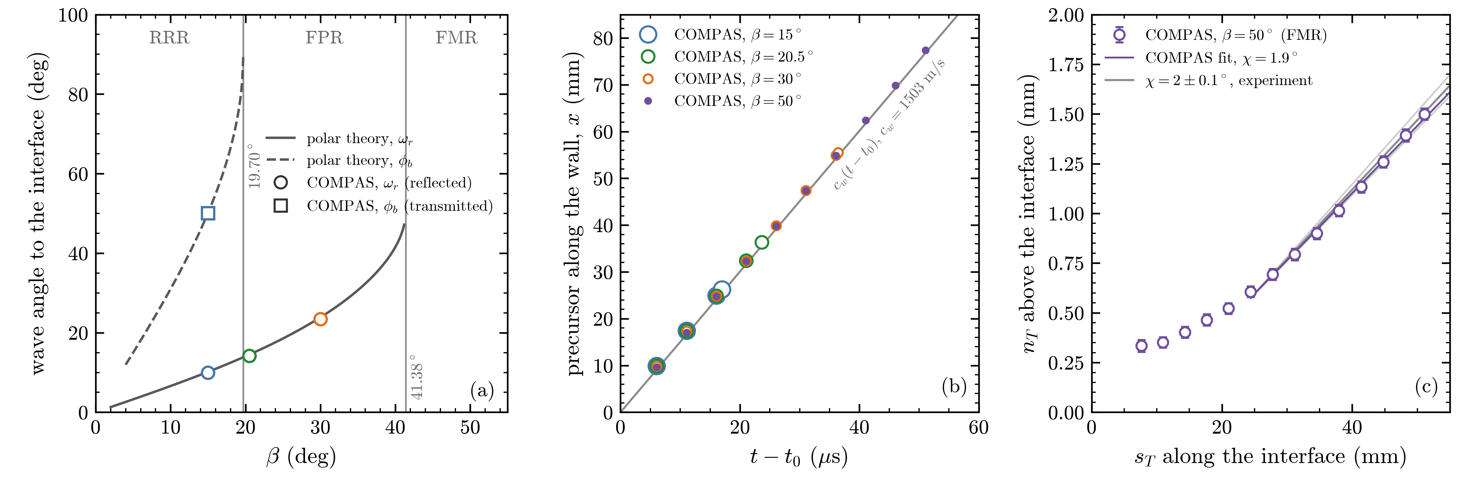
(a) Angles of the waves to the interface against \(\beta\): polar theory for the reflected shock of a regular reflection in the air, \(\omega_r\) (solid), and for the transmitted shock of RRR, \(\phi_b\) (dashed), and COMPAS (symbols). The gray vertical lines are the RRR limit, \(19.70^\circ\), and detachment in the air, \(41.38^\circ\). (b) Leading edge of the precursor along the bottom wall (symbols), against a wave that leaves the apex at \(c_w\) when the incident shock reaches it (gray line). (c) Triple point of the \(50^\circ\) run, at \(s_T\) along and \(n_T\) above the interface, with the line fitted over the second half of the run, \(\chi = 1.9^\circ\), and the \(2 \pm 0.1^\circ\) measured in the experiment (gray lines).

The runs follow the paper’s sequence: RRR at \(15^\circ\), FPR at \(30^\circ\), and FMR at \(50^\circ\), with a short Mach stem at the interface over a precursor far ahead in the water. At \(20.5^\circ\), just past the RRR limit, the transmitted wave is curved and meets the interface nearly at right angles, but its front runs along the interface at close to \(c_w\), faster than the refraction point: an FPR just past the transition, as polar theory gives and as the paper classifies its own simulation at \(20^\circ\). analysis/polar.py puts the RRR limit at \(19.70^\circ\) (the paper’s \(19.71^\circ\)), and the measured angles fall on the polar curves to within about \(0.4^\circ\) for the reflected shock and \(0.1^\circ\) for the transmitted shock. At every angle the precursor runs along the wall at the sound speed of the water, 1502 to 1507 m/s, even at \(50^\circ\), where the refraction point moves at only 662 m/s. The triple point of the \(50^\circ\) run moves at \(1.9^\circ\) to the interface, within the \(2 \pm 0.1^\circ\) measured in the experiment.

Single-mode Richtmyer-Meshkov instability

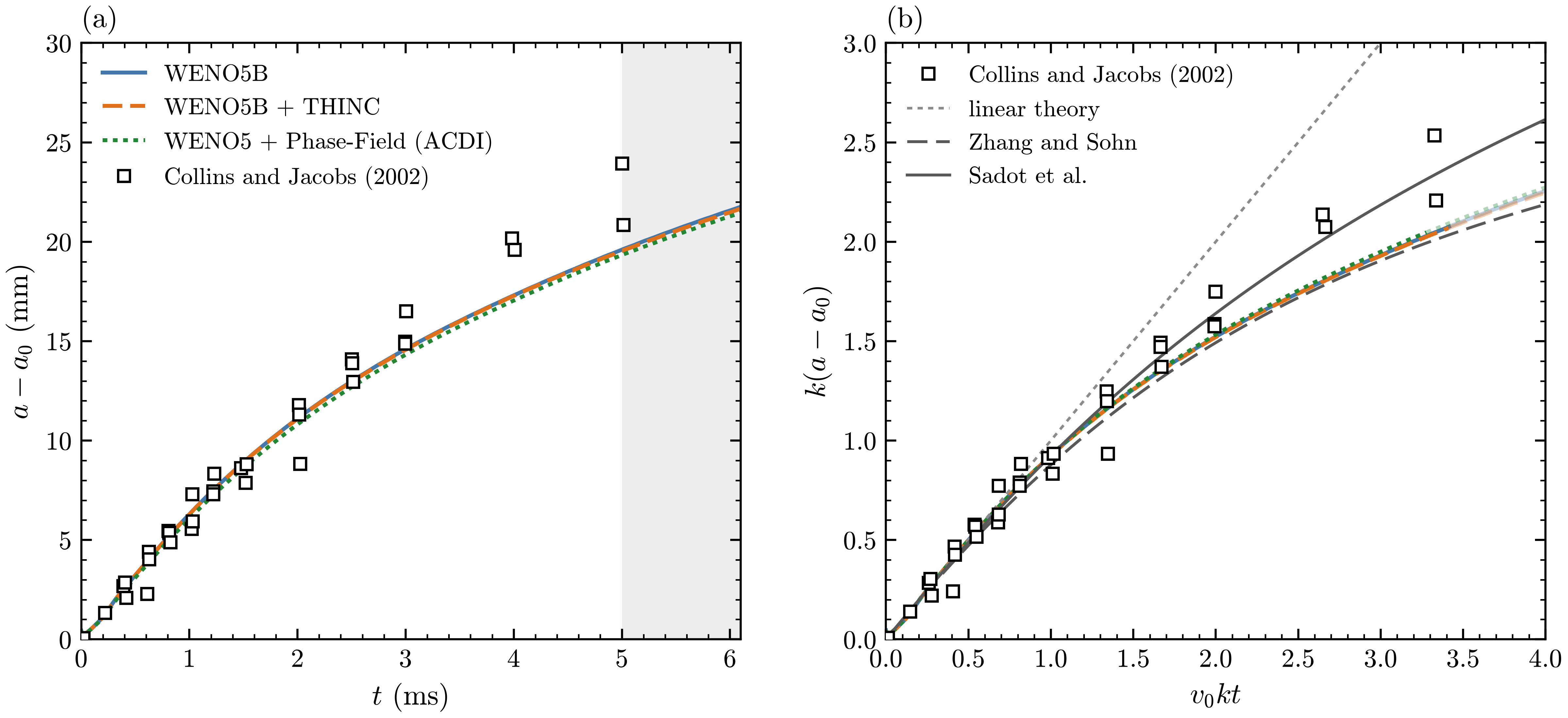
Single-mode Richtmyer-Meshkov instability, \(M_s = 1.21\), against Collins and Jacobs (2002). (a) Amplitude growth \(a - a_0\) against the time \(t\) after the shock reaches the interface, for WENO5B, WENO5B + THINC and WENO5 + Phase-Field (ACDI), with their measurements (squares); after 5 ms (shaded) the interface in the experiment is reaccelerated. (b) The same in the scaled variables \(k(a - a_0)\) and \(v_0 k t\), each run scaled with its own \(v_0\), against linear theory, the Pade model of Zhang and Sohn and the model of Sadot et al. (eqs. (6), (9) and (10) of Collins and Jacobs), with \(A = 0.62\) and \(k a_0 = 0.194\).

Collins and Jacobs (J. Fluid Mech. 464, 2002) measured single-mode Richtmyer-Meshkov growth with planar laser-induced fluorescence. A shock runs from air, seeded with acetone, into SF\(_6\) across an interface of wavelength \(\lambda = 59.33\) mm and amplitude \(a_0 = 1.83\) mm. At \(M_s = 1.21\) they measured an initial growth rate \(v_0 = 6.28 \pm 0.60\) m/s, with Atwood numbers of 0.604 before the shock and 0.625 after it. The symbols are their points of Fig. 14.

exec/_Tests/RichtmyerMeshkov-5Eq is run with the parameters of the experiment on the command line, in units of the wavelength, \(10^5\) Pa and the air-acetone density: air-acetone is an ideal gas with \(\gamma = 1.276\), and SF\(_6\) one with \(\gamma = 1.093\) and density 4.0666. Half a wavelength is simulated between symmetry planes at the crest and the trough, in a tube from a wall at \(y = -16\) to an outflow at \(y = 2\), with four levels of refinement, 512 cells per wavelength at the finest. The runs use HLLC and TVD-RK3: WENO5B alone and with THINC, from an interface \(\eta = 0.5\) finest cells wide, and WENO5 with the explicit ACDI Phase-Field, from \(\eta = 2\):

cd exec/_Tests/RichtmyerMeshkov-5Eq && make -j4
mkdir -p plot/CJ/base plot/CJ/thinc plot/CJ/pf
CJ=(prob.EOS.gamma_1=1.276 prob.EOS.gamma_2=1.093 prob.rho1=1.0 prob.rho2=4.0666
    prob.Mach=1.21 prob.a0=0.03084
    "geometry.prob_lo=0 -16 -1" "geometry.prob_hi=0.5 2 1" "amr.n_cell=16 576 8"
    amr.max_level=4 amr.max_grid_size=32 stop_time=28.0 run.user_output_int=1
    "amr.t_write=4.75259 9.26026 13.83212 18.40857 23.02170 27.56605"
    amr.t_write_interval=0.45856 amr.chk_int=-1)
mpirun -n 3 ./main2d.gnu.MPI.ex prob/inputs "${CJ[@]}" amr.case_name=./plot/CJ/base/RMI \
    FiniteVolume.Scheme=WENO5B PhaseField.Eta_Multiplier=0.5 \
    FiniteVolume.THINC=0 PhaseField.phase_field=0 > plot/CJ/base/run.log
mpirun -n 3 ./main2d.gnu.MPI.ex prob/inputs "${CJ[@]}" amr.case_name=./plot/CJ/thinc/RMI \
    FiniteVolume.Scheme=WENO5B PhaseField.Eta_Multiplier=0.5 \
    FiniteVolume.THINC=1 PhaseField.phase_field=0 > plot/CJ/thinc/run.log
mpirun -n 3 ./main2d.gnu.MPI.ex prob/inputs "${CJ[@]}" amr.case_name=./plot/CJ/pf/RMI \
    FiniteVolume.Scheme=WENO5 PhaseField.Eta_Multiplier=2.0 \
    FiniteVolume.THINC=0 PhaseField.phase_field=1 > plot/CJ/pf/run.log

stop_time = 28.0 is 6.10 ms, amr.t_write gives the times of Fig. 6 of the paper, and amr.t_write_interval a plotfile every 0.1 ms. The case writes the amplitude \(a\), half the distance between the \(\alpha_1 = 0.5\) crossings in the crest and trough columns, to out1D_RMI.csv every coarse step; \(t = 0\) is when the shock reaches the mean interface. The test suite clears plot/ in every test case it runs, so move the runs elsewhere before running it.

The three runs from shock arrival to 6 ms, from left to right WENO5B, WENO5B + THINC and WENO5 + Phase-Field (ACDI), with every patch box of AMR levels 1 to 4 on the left half of each panel. On the right half, the simulated one, the markers are the points the amplitude is measured from: the α₁ = 0.5 crossings at the top of the SF₆ spike, in the crest column (the line at x = 0), and at the bottom of the air bubble, in the trough column (the right edge); the bar between them is 2a. Below, a − a₀ of each run up to the time of the frame, in the colors of its markers, with the measurements of Collins and Jacobs (squares). Download the MP4.

Each run is measured from the \(a_0\) of a straight-line fit of its early growth, which also gives its \(v_0\), within the error bar of the measured one for all three. The runs agree with each other to a few tenths of a millimetre, follow the data at early times and lie below it later; after about 5 ms the interface in the experiment is reaccelerated, a stage outside the simulated problem. In the scaled variables the runs lie close to the Pade curve of Zhang and Sohn. The interface treatment shows in the roll-up cores: with WENO5B alone they spread into mixed material, with THINC the interface stays within about two cells but the thin sheet rolled into each core breaks into small drops from about 3 ms, and with Phase-Field the cores separate into blobs by 3 ms.

Hydrodynamic instabilities

Single-mode Rayleigh-Taylor instability

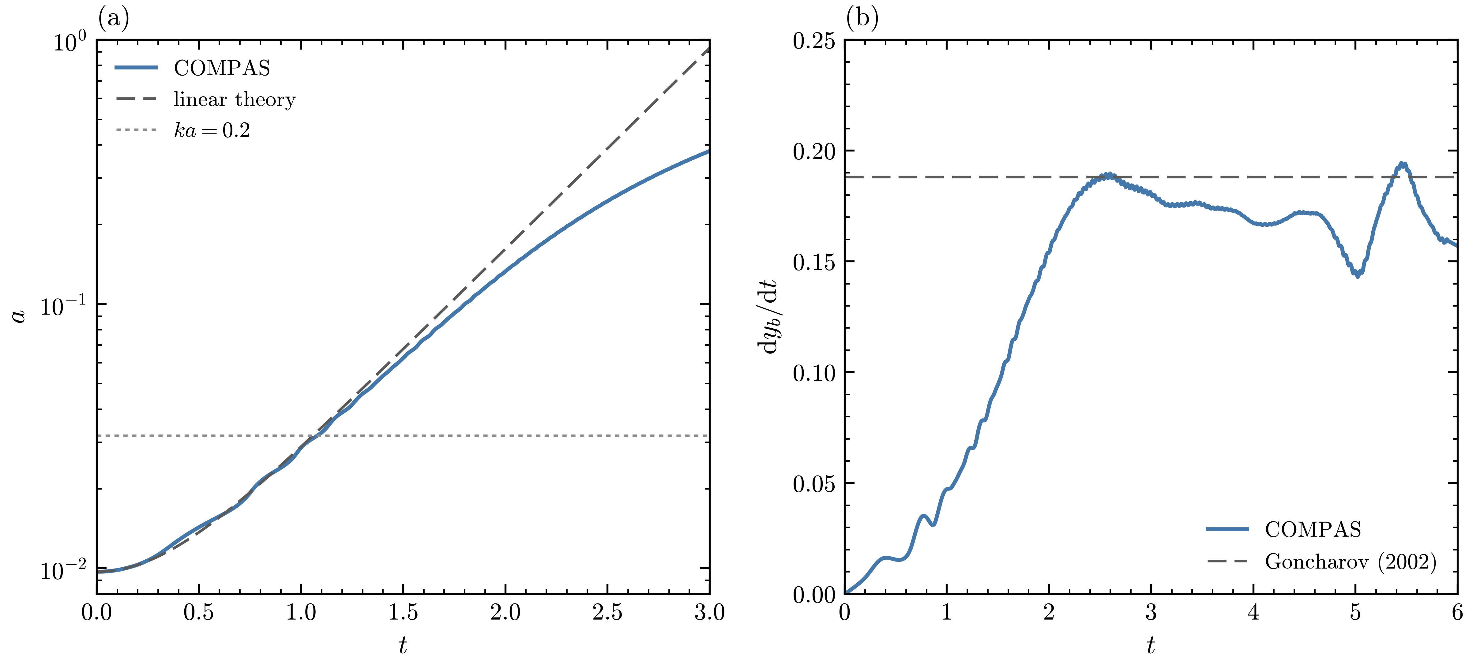
Single-mode Rayleigh-Taylor instability (\(A = 0.5\), \(k a_0 = 0.063\), MUSCL-MC + THINC). (a) Amplitude \(a = (y_b - y_s)/2\) against \(a_0\cosh\sigma t\), with the viscous linear rate \(\sigma = \sqrt{Agk + \nu^2k^4} - \nu k^2\); the dotted line marks \(ka = 0.2\), where the linear stage ends. (b) Bubble-tip velocity \(dy_b/dt\) against the terminal velocity of Goncharov (2002), \(V_b = \sqrt{2A/(1+A)\,g/(3k)}\).

exec/_Tests/RayleighTaylor (its default build, in 2D) puts a heavy fluid (\(\rho_1 = 3\)) over a light one (\(\rho_2 = 1\)), so \(A = 0.5\), under \(g = 1\), with interface \(y = a_0\cos kx\), \(k = 2\pi\). Half a wavelength is simulated between slip walls, on 64 by 512 finest cells, with MUSCL-MC, THINC and \(\mu = 0.001\); \(P_0 = 100\) keeps the flow nearly incompressible. The run sets \(a_0 = 0.01\):

cd exec/_Tests/RayleighTaylor && make -j3
mpirun -n 3 ./main2d.gnu.MPI.ex prob/inputs prob.a0=0.01 stop_time=6 amr.t_write_interval=0.05 run.user_output_int=10

The run from t = 0 to 6: the heavy-fluid volume fraction (heavy deep blue, light sand), mirrored to one wavelength. The markers are the points the amplitude is measured from, the α₁ = 0.5 crossings at the bubble tip y_b, in the bubble column (the right edge), and at the spike tip y_s, in the spike column (the line in the middle); the bar is 2a = y_b − y_s. Right: the amplitude against a₀ cosh σt and the bubble-tip velocity against the terminal velocity of Goncharov, as in the figure above, drawn up to the time of the frame. Download the MP4.

The amplitude follows \(a_0\cosh\sigma t\) until \(ka \approx 0.2\), at a rate 3 percent below \(\sigma\) (1.705 against 1.753), as expected for an interface spread over one and a half to two cells, since a diffuse interface of thickness \(L\) grows at about \(\sqrt{Agk/(1+kL)}\). The bubble tip then reaches the terminal velocity of Goncharov (Phys. Rev. Lett. 88, 2002) at \(t \approx 2.6\), and stays between 0.76 and 1.03 times it while vortices roll up along the spike and inside the bubble, which the potential-flow model does not include.

Compressible Kelvin-Helmholtz instability

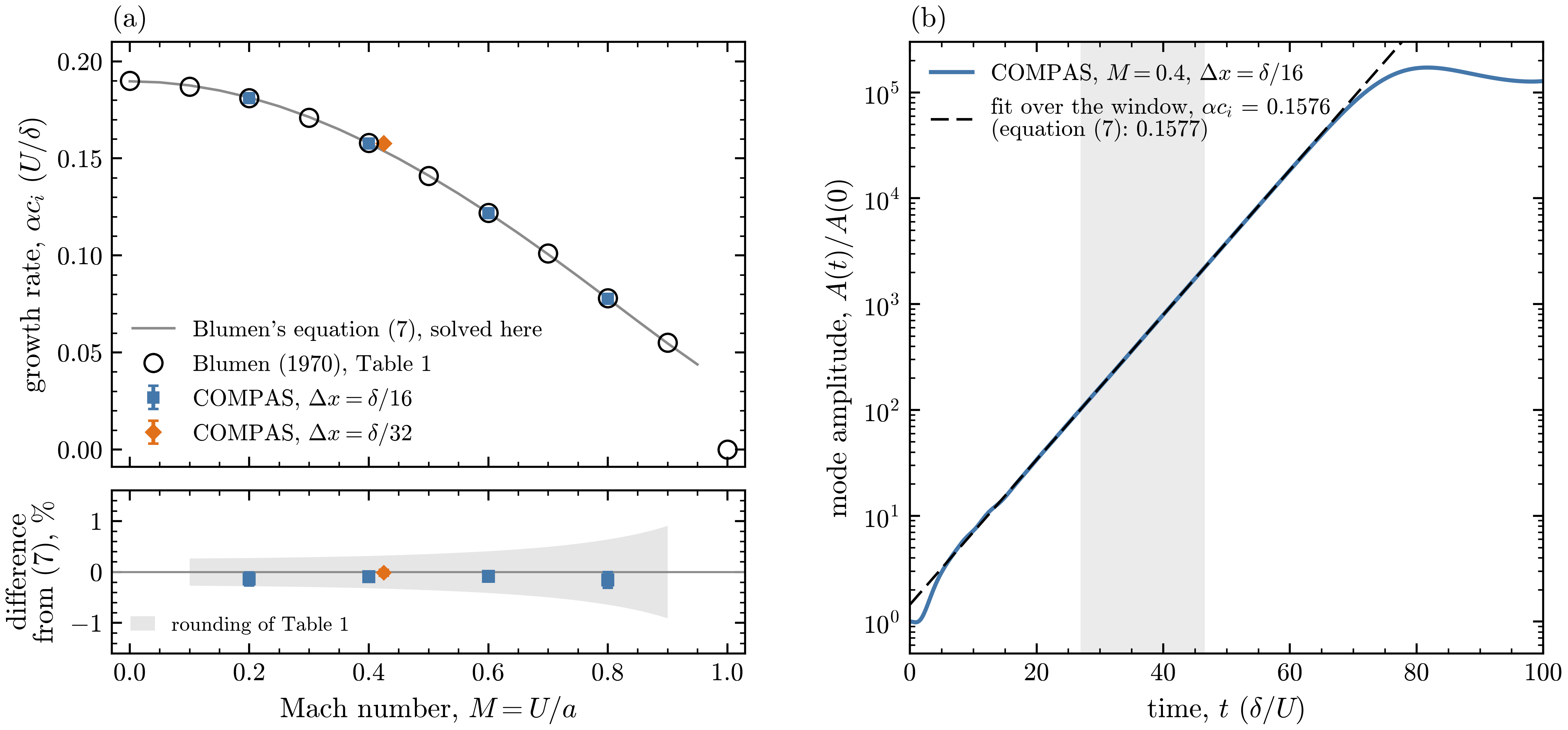
(a) Growth rate \(\alpha c_i\) of the fastest-growing mode against the Mach number \(M = U/a\), from Blumen’s Table 1 (circles), his equation (7) solved by analysis/blumen.py (line), and COMPAS with cells of \(\delta/16\), and of \(\delta/32\) at \(M = 0.4\); below, the difference from equation (7), with the rounding of Table 1 shaded. (b) The amplitude of the seeded mode at \(M = 0.4\). The gray band is the fit window (\(t = 27.0\) to 46.5 \(\delta/U\)) and the dashed line the exponential fitted over it, \(\alpha c_i = 0.1576\) against 0.1577 from equation (7).

Blumen (J. Fluid Mech. 40, 1970) computed the linear stability of the shear layer \(u = U\tanh(y/\delta)\) in an inviscid ideal gas at uniform pressure and density. His Table 1 gives at each Mach number the wavenumber \(\alpha_{\max}\) of the fastest-growing mode, which is stationary, and its growth rate \(\alpha c_i\), which falls from 0.190 at \(M = 0\) to 0.078 at \(M = 0.8\). analysis/blumen.py solves his equation (7) by shooting and reproduces every rate of the table.

exec/KelvinHelmholtz-5Eq sets up this layer with \(\rho = 1\), \(U = \delta = 1\) and \(p = 1/(\gamma M^2)\), \(\gamma = 1.4\), in one wavelength \(2\pi/\alpha_{\max}\), periodic in \(x\), between slip walls about \(20\delta\) from the layer, and seeds it with one small divergence-free mode, \(v = 10^{-5}\,U\sin(\alpha_{\max} x)\,\mathrm{sech}(y/\delta)\). Both materials are the same gas at the same density, so \(\alpha_1 = [1 + \tanh(y/\delta)]/2\) is a passive tracer. Two levels of refinement cover fixed bands around the layer, cells of about \(\delta/16\), and the runs use WENO5, HLLC and TVD-RK3. The inputs are set for \(M = 0.4\):

cd exec/KelvinHelmholtz-5Eq && make -j3
mpirun -n 3 ./main2d.gnu.MPI.ex prob/inputs
python3 analysis/growth.py 0.2:0.2:16.27:data/mode_M0.2.csv 0.4:0.4:16.14:data/mode_M0.4.csv \
    0.6:0.6:16.02:data/mode_M0.6.csv 0.8:0.8:15.99:data/mode_M0.8.csv \
    0.4-d32:0.4:32.29:data/mode_M0.4-d32.csv --out growth_rates.csv --figure kh_growth.png

Each run writes the amplitude \(A\) of the seeded Fourier mode of \(v\), integrated over \(y\), to mode.csv. data/ holds the histories of the seven runs of this section, and data/README.txt gives the command of each: \(M = 0.2\), 0.6 and 0.8, a third level at \(M = 0.4\), and the sharp tracer below. analysis/growth.py fits the slope of \(\ln A\) from \(A = 100\,A(0)\) to the time the largest \(|v|\) reaches \(0.01\,U\), with an uncertainty from the two halves of that window and from moving its ends; the second command redraws the figure from data/.

The M = 0.4 run from t = 0 to 95 δ/U. Left: the passive tracer α₁ over one wavelength, with contours of the transverse velocity v at ±0.25, 0.5 and 0.75 of its largest magnitude in the frame (dashed where v < 0). After the sound waves of the first few δ/U, the contours settle into the eigenmode, which grows in place, far too small to move the tracer, until it rolls the layer up after t ≈ 60. Right: the amplitude A of the seeded Fourier mode of v up to the time of the frame, with the fit window (gray band), the fitted exponential (dashed) and, two decades lower, a line with the rate of Blumen's equation (7). Download the MP4.

At all four Mach numbers the growth rate agrees with Table 1 to within its rounding, and with equation (7) to within 0.2 percent; halving the cells at \(M = 0.4\) brings it within its uncertainty. The mode keeps its phase and grows without oscillation, so it is stationary, like those of the table. It stays on the fitted exponential until \(|v|\) is a few percent of \(U\), and then saturates as the layer rolls up into a single vortex.

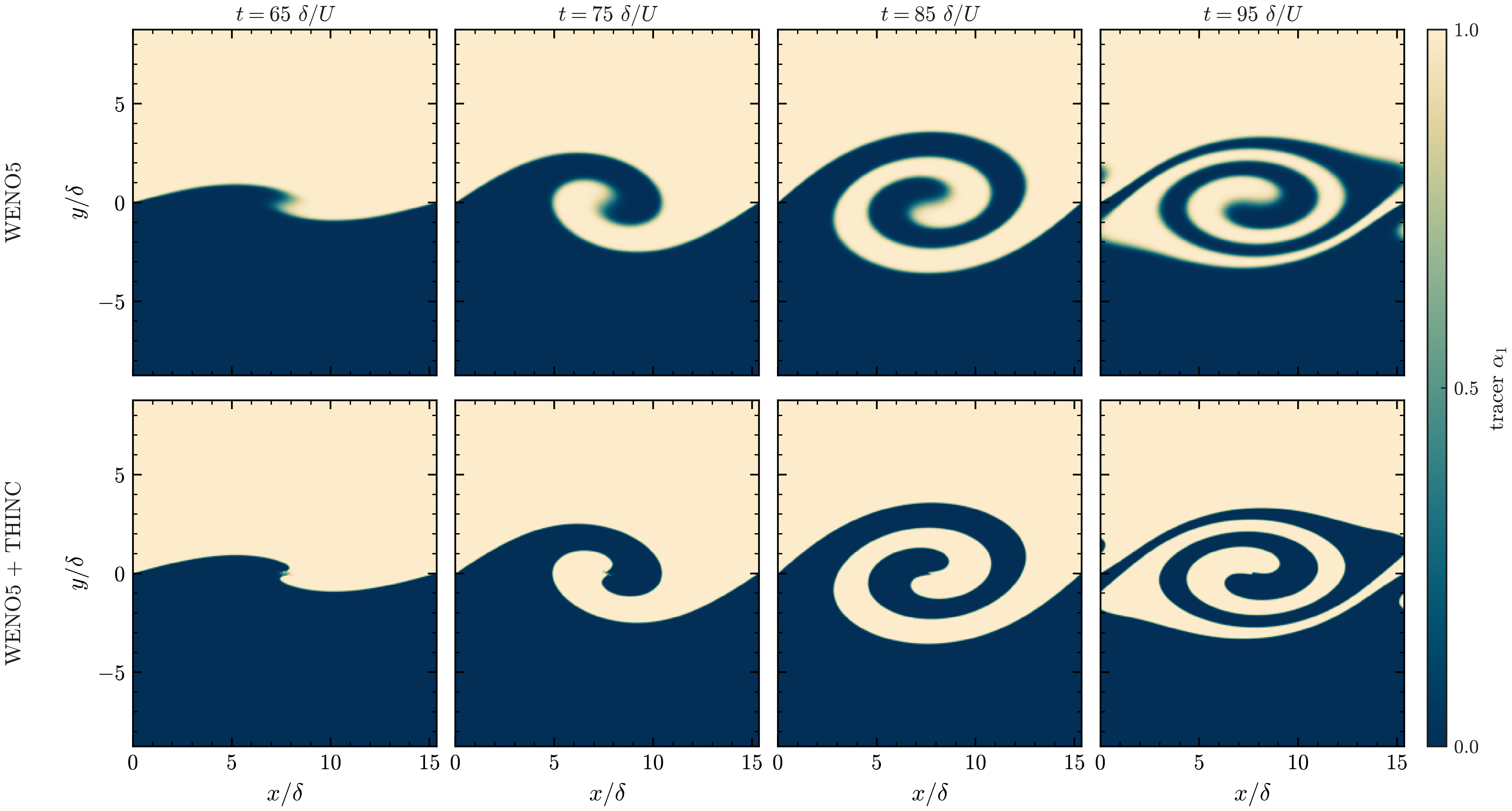
A sharp tracer, \(\alpha_1 = [1 + \tanh(y/w)]/2\) with \(w = 0.0619\,\delta\), one finest cell, in the same \(M = 0.4\) flow at \(t = 65\) to 95 \(\delta/U\), with WENO5 (top row) and WENO5 + THINC (bottom row).

A tracer one finest cell wide (prob.tracer_width) compares the interface treatments in the same flow; the growth rate is the same with THINC, \(0.1576 \pm 0.0001\). Its 5 to 95 percent thickness (scripts/postprocess.py interface), 4.0 finest cells at \(t = 0\), grows to 5.4 cells by \(t = 95\) with WENO5 alone and stays at 1.6 cells with THINC, with \(\alpha_1\) within \([0, 1]\) to about \(4 \times 10^{-5}\). With both schemes the tracer stays in one piece through the roll-up, apart from a few mixed cells at the inner tip of the spiral.